A hierarchical probabilistic U-Net for modeling multi-scale ambiguities
Notes
Highlights
- The objective of this paper is to develop a generative model for semantic segmentation able to learn complex-structured conditional distributions.
- The innovation comes from the modelling of a coarse-to-fine hierarchy of latent variables to improve fidelity to fine structures in the model’s samples and reconstructions.
- The proposed framework is capable of modelling distributions over segmentations with factors of variations across space and scale.
Method
Appetizer
The following animation illustrates the capacity of the method in modelling complex structured distributions across scales.
Architecture
- The architecture is based on the conditional VAE whose details are provided in the following tutorial.
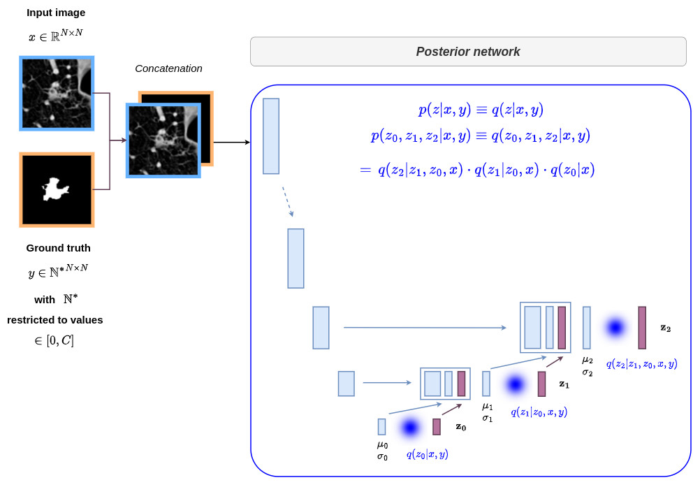
- The main innovation comes from the following hierarchical modelling of the latent space:
In the particular case where \(L=2\), the above equation can be put in the following form:
\[p\left(\boldsymbol{z} \vert x\right) = p\left(z_2 \vert z_1,z_0,x\right) \cdot p\left(z_1 \vert z_0,x\right) \cdot p\left(z_0 \vert x\right)\] \[q\left(\boldsymbol{z} \vert x,y\right) = q\left(z_2 \vert z_1,z_0,x,y\right) \cdot q\left(z_1 \vert z_0,x,y\right) \cdot q\left(z_0 \vert x,y\right)\]Taking into account the hierarchical modelling, a new ELBO objective with a relative weighting factor \(\beta\) was formulated as follows (the corresponding demonstration is given at the end of this post):
\[\mathcal{L}_{ELBO} = \mathbb{E}_{\boldsymbol{z}\sim q(\boldsymbol{z} \vert x,y)} [CE\left( y,\hat{y}\right)] + \beta \cdot \sum_{i=0}^{L} \mathbb{E}_{z_{i-1}\sim \prod_{j=0}^{i-1} q(z_j \vert z_{<j},x,y)} [D_{KL}(q(z_i \vert z_{<i},x,y) \parallel p(z_i \vert z_{<i},x))]\]The authors observed that the minimization of \(\mathcal{L}_{ELBO}\) leads to sub-optimal results. For this reason, they used the recently proposed \(GECO\) loss (GECO stands for Generalized ELBO with Constrained Optimization):
\[\mathcal{L}_{GECO} = \lambda \cdot \left( \mathbb{E}_{\boldsymbol{z}\sim q(\boldsymbol{z} \vert x,y)} [CE\left( y,\hat{y}\right)] - \kappa \right) + \sum_{i=0}^{L} \mathbb{E}_{z_{i-1}\sim \prod_{j=0}^{i-1} q(z_j \vert z_{<j},x,y)} [D_{KL}(q(z_i \vert z_{<i},x,y) \parallel p(z_i \vert z_{<i},x))]\]where \(\kappa\) is chosen as the desired reconstruction error and \(\lambda\) is a Lagrange multiplier that is updated as a function of the exponential moving average of the reconstruction contraint.
This formulation initially puts high pressure on the reconstruction and once the desired \(\kappa\) is reached it increasingly moves the pressure over on the KL-terms.
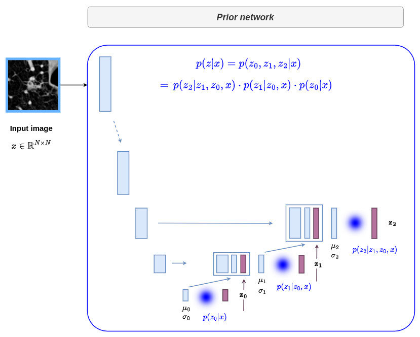
Finally, the prior and the generator networks are based on the same U-Net architecture, which results in parameter and run-time savings.
The overall architecture is given below:
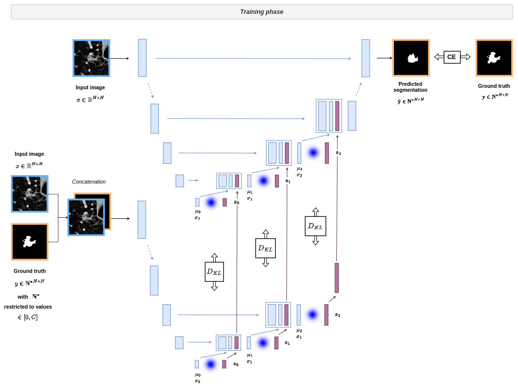
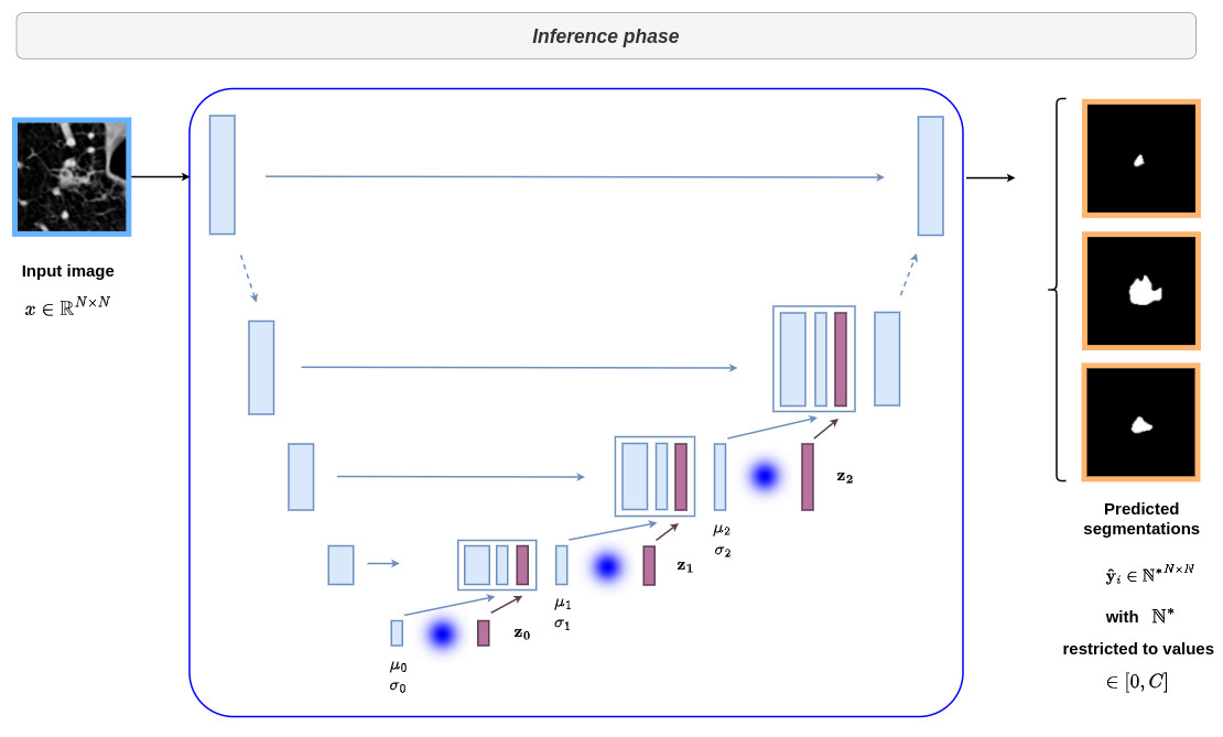
This architecture can be difficult to understand at first sight. Therefore I show below the different parts of the network with reference to the formalism of the conditional VAE

Implementation details
- U-Nets are composed by res-blocks.
Without the use of res-blocks, the KL-terms between distributions at the begining of the hierarchy often become 0 early in the training, essentially resulting in uninformative and thus unused latents.
- The number of latent scales is chosen empirically to allow for a sufficiently granular effect of the latent hierarchy.
Distribution agreement
To assess the quality of the generative network, it is necessary to measure the agreement between two distributions based on samples only. The following two metrics have been used:
- Generalized Energy Distance
where \(d\) is a distance measure, \(y\) and \(y'\) are independent samples from the ground truth distribution \(P_{gt}\), \(\hat{y}\) and \(\hat{y}'\) are independent samples from the predicted distribution \(P_{out}\). The distance measure is based on the \(\text{IoU}\) metric and is defined as follows: \(d(x,y)=1-\text{IoU}(x,y)\).
When the model’s samples poorly match the ground truth samples, this metric rewards sample diversity regardless of the samples’ adequacy :(
- Hungarian-matched \(\text{IoU}\)
The Hungarian algorithm finds the optimal 1:1-matching between the objects of two sets. \(\text{IoU}(y,\hat{y})\) was used to determine the similarity between two samples. Finally, the average \(\text{IoU}\) of all matched pairs was used as the Hungarian-matched \(\text{IoU}\) metric.
Contrary to \(D^2_{GED}\), higher values mean better performances.
Reconstruction fidelity: \(\text{IoU}_\text{rec}\)
- The reconstruction fidelity is defined as an upper bound on the fidelity of the conditional samples.
- It measures how well the model’s posteriors are able to reconstruct a given segmentation in terms of the IoU metric.
where \(S\left( x,\mu_{post}(x,y) \right)\) corresponds to the segmentation result computed from the posterior network.
Results
LIDC-IDRI dataset
- 1010 2D+slices CT scan of lungs with lesions
- For each scan, 4 radiologists (from a total of 12) provided annotation masks for lesions that they independently detected
- the CT scans were resampled to \(0.5 \, \text{mm} \times 0.5 \, \text{mm}\) in-plane resolution and cropped 2D images (\(180 \times 180\) pixels) centered at the lesion positions.
- This resulted in \(8882\) images in the training set, \(1996\) images in the validations set and \(1992\) images in the test set.
- Because the experts can disagree, up to 3 masks per image can be empty.
- A number of latent scales of 4 (\(L=3\)) was experimentally chosen.
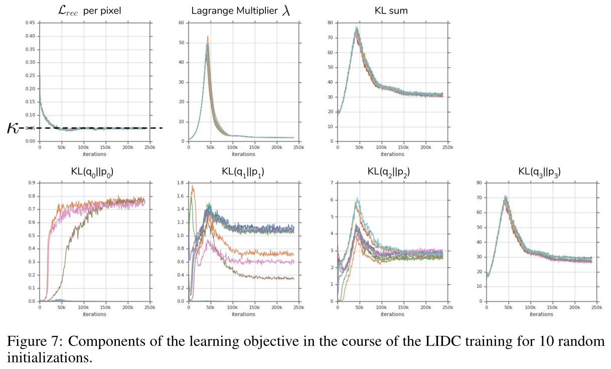
- A GECO loss using \(\kappa=0.05\) was used.
The figure below first shows the evolution of the different parts of the loss over time for 10 random initializations.
The table below provides the overall results obtained in terms of \(\text{IoU}_\text{Rec}\) and Hungarian-matched \(\text{IoU}\). Subset B corresponds to cases where 4 graders agree on the presence of an abnormality.

The next figure displays the results obtained on two different cases. sPU-Net corresponds to the Probabilistic U-Net method.

In order to explore how the model leverages the hierarchical latent space decomposition, the predicted means \(\mu_{prior}\) can be used for some scales instead of sampling. The figure below (Fig. 3a) shows samples for the given CT scans resulting from the process of sampling from the full hierarchy, i.e. from 4 scales in this case. Fig. 3b,c show the resulting samples when sampling from the most global or most local scale only.

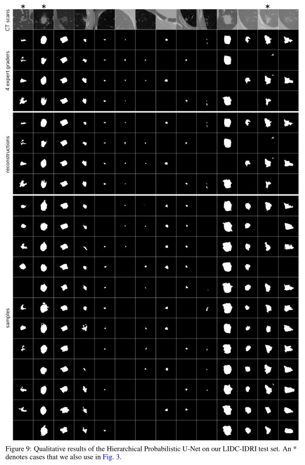
The last figure below shows other examples of segmentations generated from the proposed method.
Conclusions
- The work proposed a significantly improved version of the probabilistic U-Net
- It allows to model complex-structured conditional distribution thanks to a coarse-to-fine hierarchy of latent variables
Appendix
KL-divergence of the proposed model
\[D_{KL}\left(q(\boldsymbol{z} \vert x,y)\parallel p(\boldsymbol{z} \vert x)\right) = \mathbb{E}_{\boldsymbol{z}\sim q(\boldsymbol{z} \vert x,y)}\left[ log\left(q(\boldsymbol{z} \vert x,y)\right) - log\left(p(\boldsymbol{z} \vert x)\right) \right]\] \[=\int_{z_0,\cdots,z_L} q(\boldsymbol{z} \vert x,y) \cdot \left[ log\left(q(\boldsymbol{z} \vert x,y)\right) - log\left(p(\boldsymbol{z} \vert x)\right) \right] dz_0 \ldots dz_L\] \[=\int \prod_{j=0}^{L}q(z_j \vert z_{<j},x,y) \cdot \left[ log\left(\prod_{i=0}^{L}q(z_i \vert z_{<i},x,y)\right) - log\left(\prod_{i=0}^{L}p(z_i \vert z_{<i},x)\right) \right] dz_0 \ldots dz_L\] \[=\int_{z_0,\cdots,z_L} \prod_{j=0}^{L}q(z_j \vert z_{<j},x,y) \cdot \sum_{i=0}^{L}\left[ log\left(q(z_i \vert z_{<i},x,y)\right) - log\left(p(z_i \vert z_{<i},x)\right) \right] dz_0 \ldots dz_L\] \[=\sum_{i=0}^{L} \int_{z_0,\cdots,z_L} \prod_{j=0}^{L}q(z_j \vert z_{<j},x,y) \cdot \left[ log\left(q(z_i \vert z_{<i},x,y)\right) - log\left(p(z_i \vert z_{<i},x)\right) \right] dz_0 \ldots dz_L\]Using
\[\int_{z_0,\cdots,z_L} \phi(z_i) \prod_{j=0}^{L} q(z_j \vert z_{<j},x,y) dz_0,\ldots,dz_L=\int_{z_0,\cdots,z_i} \phi(z_i) \prod_{j=0}^{i} q(z_j \vert z_{<j},x,y) dz_0,\ldots,dz_i\](this relationship is demonstrated at the end of this post, a big thank to Lucas Braz for his help !)
We have
\[=\sum_{i=0}^{L} \int_{z_0,\cdots,z_i} \prod_{j=0}^{i}q(z_j \vert z_{<j},x,y) \cdot \left[ log\left(q(z_i \vert z_{<i},x,y)\right) - log\left(p(z_i \vert z_{<i},x)\right) \right] dz_0 \ldots dz_i\] \[=\sum_{i=0}^{L} \int \prod_{j=0}^{i-1} q(z_j \vert z_{<j},x,y) \, \underbrace{q(z_i \vert z_{<i},x,y) \cdot \left[ log\left(q(z_i \vert z_{<i},x,y)\right) - log\left(p(z_i \vert z_{<i},x)\right) \right]}_{D_{KL}(q(z_i \vert z_{<i},x,y) \parallel p(z_i \vert z_{<i},x))} dz_0 \ldots dz_i\] \[=\sum_{i=0}^{L}\mathbb{E}_{z_{i-1}\sim \prod_{j=0}^{i-1} q(z_j \vert z_{<j},x,y)} [D_{KL}(q(z_i \vert z_{<i},x,y) \parallel p(z_i \vert z_{<i},x))]\]