TreeDiffusion: Hierarchical Generative Clustering for Conditional Diffusion
Notes
- Link to the code here
Highlights
- Extension of TreeVAE by adding a diffusion model
- Controlling image synthesis based on learned clusters
- Better reconstruction quality
- Evaluation on
MNIST,FashionMNIST,CIFAR-10,CelebA, andCUBICC(images of birds)
Overall idea
- Two-stage framework
- TreeVAE
- Get a structured hierarchical latent representation (from root to leaf) from a TreeVAE
- Process the nodes with a path encoder to create the conditioning signal
- DDIM
- Denoising Diffusion Implicit Model using the path encoder as conditioning to generate cluster-conditional samples
In treeVAE, multiple decoders were used to reconstruct the images. Here, the DDIM serves as the reconstruction model
- Denoising Diffusion Implicit Model using the path encoder as conditioning to generate cluster-conditional samples
Methods
TreeVAE Reminder
- The full post is available here
- The network starts with a root and two child nodes and optimize the ELBO for a fixed number of epochs
- Then it picks the leaf with the highest sample count and split it by adding two child nodes to promote balanced leaves
- Unchanged parts are frozen and only the subtree formed by the new leaves are trained.
-
The processus alternates between expansion and localized training until reaching the target depth or number of leaves (hyperparameters)
- \(\mathbb{V}\) represents the nodes of the tree
- \(\textbf{z}_0,...,\textbf{z}_v\) are stochastic latent variables of each node
- A given sample traverses the tree from root \(\textbf{z}_0\) to a leaf node \(\textbf{z}_l\)
- The decisions of moving to either child node are \(c_i\) for each non-leaf node \(\textit{i}\). They follow a Bernoulli distribution, where \(c_i = 0\) corresponds to the left child
- \(\mathcal{P}_l\) is the path or the sequence of nodes from the root to one leaf \(\textit{l}\)
- \(z_{\mathcal{P}_l} = \left\{ z_i \mid i \in \mathcal{P}_l \right\}\) is the set of latent embeddings for each node in the path \(\mathcal{P}_l\)
- The generative model is defined by :
- The inference model is defined by :
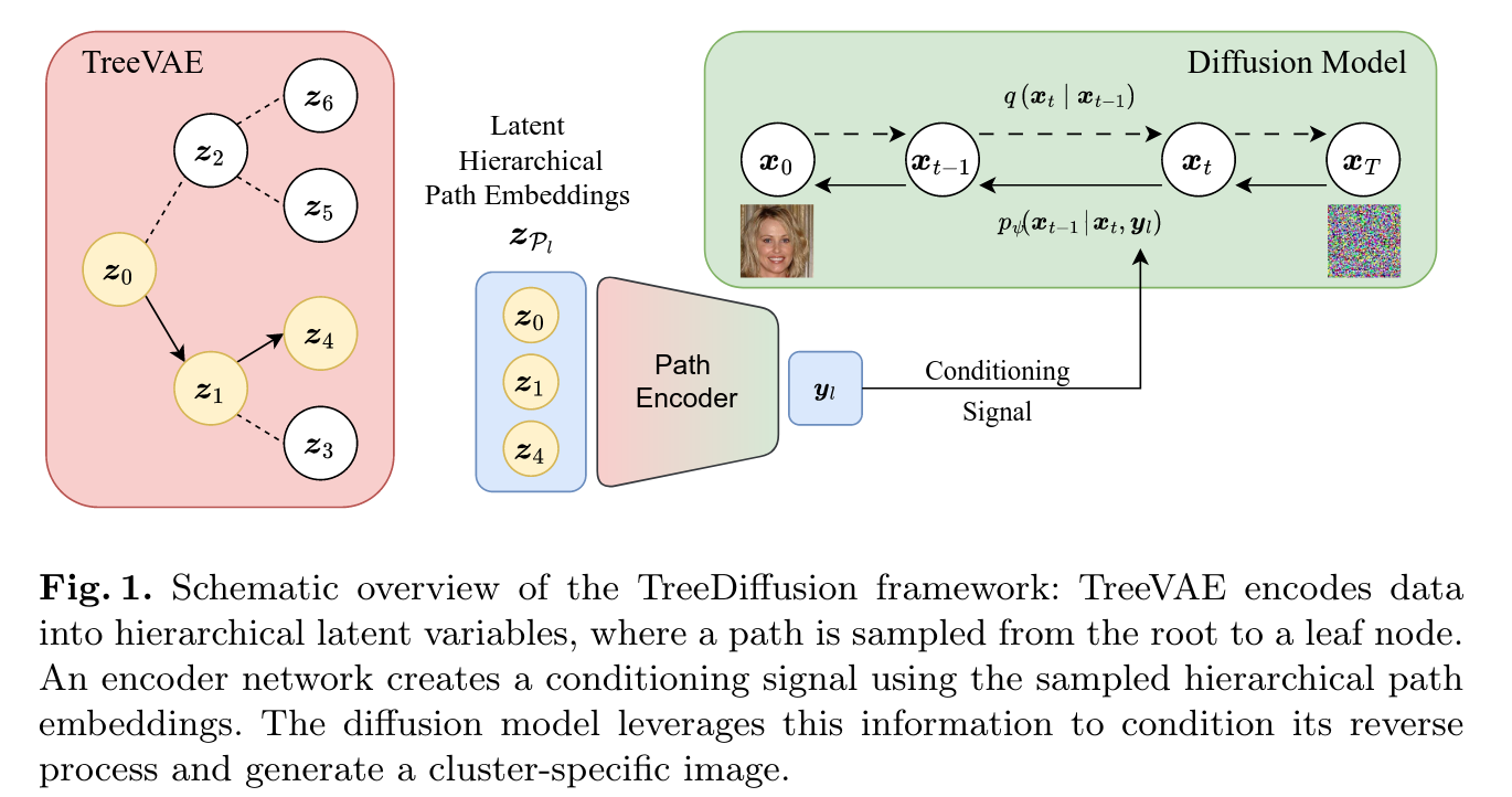
TreeDiffusion
- DDPM tutorial is available here
- Equations remain the same for the forward process
- For the reverse process, first, a path is sampled from the root to a leaf node \(\textit{l}\)
A sequence of stochastic transformations is applied to the root embedding along this path
- The hierarchical conditioning information is derived from \(\textbf{z}_{\mathcal{P}_l}\)
- These embeddings are processed by a dedicated path encoder which aggregates the information to produce the conditioning signal \(\textbf{y}_l\) :
- \(f_{embed}\) and \(f_{node}\) are implemented as projection blocks consisting of two MLP layers with a SiLU activation in-between (they are jointly trained with the diffusion model)
- Link of the architecture here
For each node in the path, its embedding and corresponding node index are projected independently into the time embedding dimension of the U-Net decoder.
Currently, sampling is limited to paths originating from the root
- The reverse process is like a DDPM using the \(\textbf{y}_l\) signal as the conditioning term
- They used DDIM to accelerate inference
TreeVAE + Diffusion
- Similar method than DiffuseVAE [1]
- You take the output of a VAE-based model and you apply a diffusion model on it to get better reconstructed samples
- You keep the representation of a VAE while improving the reconstruction part
- TreeVAE + Diffusion is the same process than DiffuseVAE: You take the reconstructed image from the decoder of one leaf and you give it to a diffusion model to refine the reconstruction (in this case, there is no condition on any latent information from the hierarchical structure)
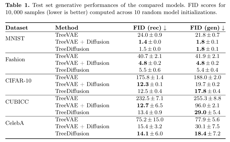
Results
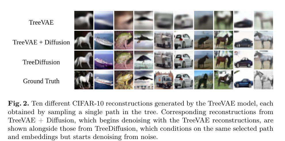
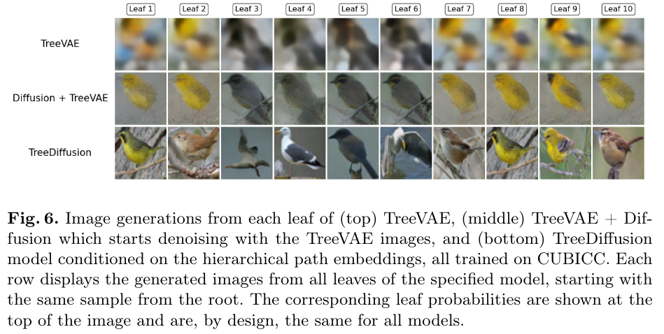
- The naive approach performs better at image reconstruction rather than generation
TreeVAE + Diffusion model begins denoising from TreeVAE reconstructions, thereby making it highly dependent on the reconstruction quality provided by TreeVAE.
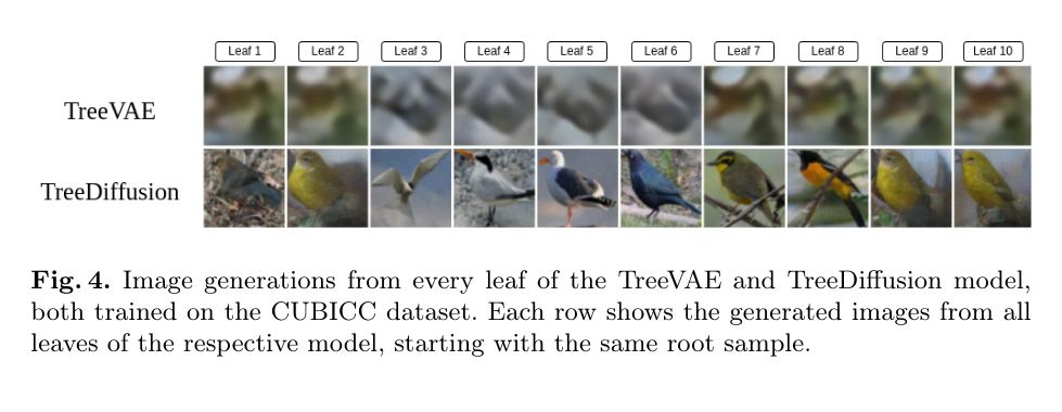
- TreeDiffusion achieves a better balance between reconstruction and generation quality
- For each generation, they sample the root embedding, then select a path through the tree and refine the representations along this path until a leaf is reached
- TreeDiffusion produces sharper images for all clusters but also generates a greater diversity of images
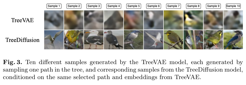
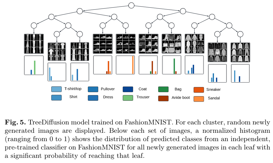
- To quantitatively evaluate cluster retention in generated images, a classifier is trained on the original labeled dataset and then used to predict the classes of TreeDiffusion-generated samples
- The “purity” of leaf nodes is assessed by examining whether generated samples are consistently classified into one or a small number of classes
- High classification consistency indicates that TreeDiffusion effectively preserves hierarchical cluster information in its outputs
- Conditioning on hierarchical representations improves cluster-specific generative quality
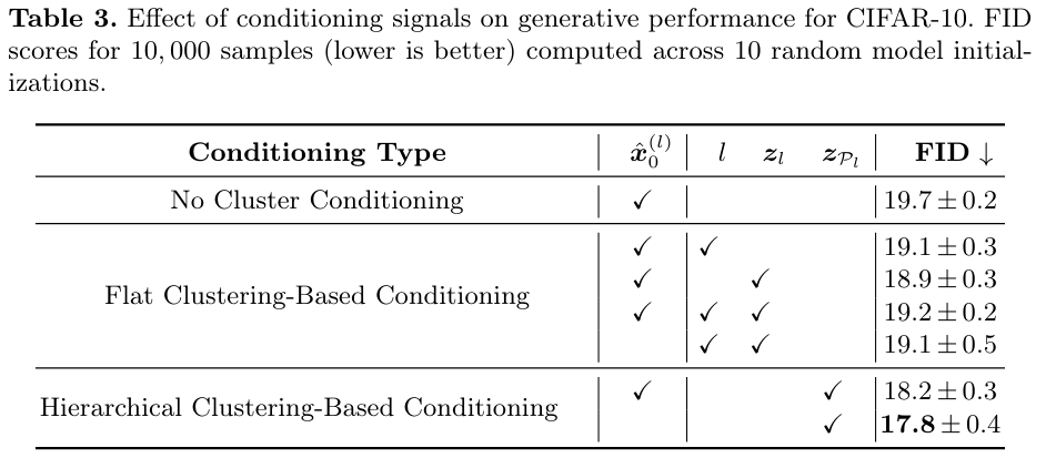
- Ablation study on the conditional information \(\textbf{y}_l\)
Note that the first row in the table represents the TreeVAE + Diffusion model from the previous experiments, whereas the last row corresponds to the proposed TreeDiffusion method
Conclusions
- TreeVAE provides effective hierarchical clustering representations, while the diffusion model enables high-quality image generation.