Highlights

The authors modelize the bias of graph data into two components : attribute bias and structure bias
They suggest a framework for a model-agnostic bias mitigation based on the minimization of the Wasserstein distance

Introduction

This post assumes that the reader is familiar with the basic concepts of graph neural networks and optimal transport. Both topics were covered in previous tutorials : Introduction to Optimal Transport and Introduction to Graph Neural Networks
Assuming that a biased graph dataset is used to train a GNN, a “sensitive information” refers to any data present in the dataset that could be used for the predictions, leading to an unwanted discrimination
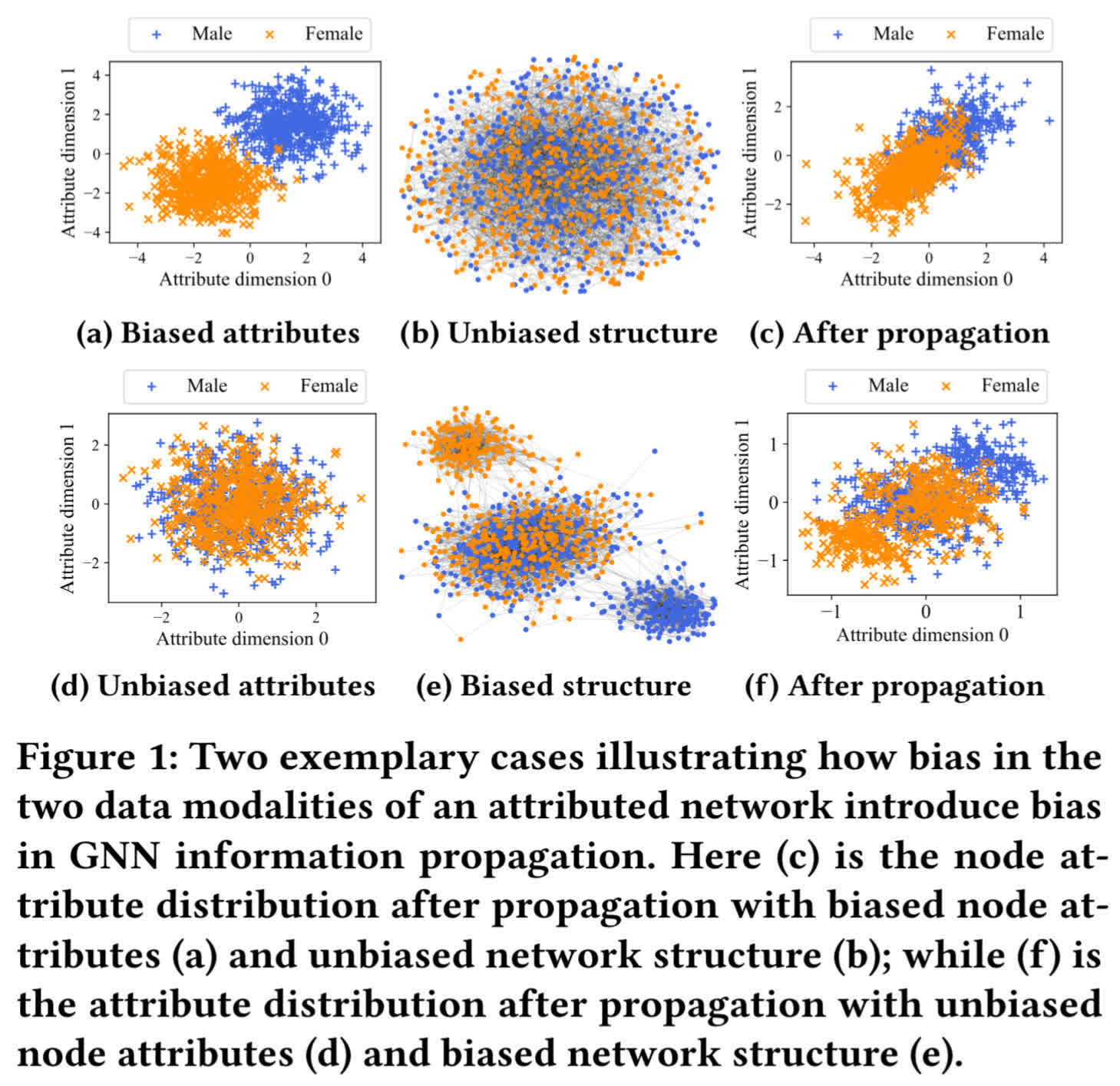
To introduce the issue, the authors generates a synthetic graph (for a node-classification context) modeling a social network. Nodes represent individuals, and edges represent any connexions between the nodes (you can think of a mutual follow on a social media).
Here, we consider a task that does not require the gender of the individual (think of a recommendation algorithm). Thus in this context, the gender is considered as the sensitive information, and needs to be hidden to the GNN
On the figure below, the first row shows that biased attributes in an unbiased structure propagate biased attributes to the next layer of the GNN. The second row shows that unbiased attributes in a biased structure also propagate biased attributes to the next layer of the GNN
Hence, the intuition of the paper is that a graph debiasing method needs to mitigate both the attribute bias of the nodes, but also the structure bias of the nodes

Notations

Let \(G = (A, X)\) be an undirected attributed network. Here \(A \in \mathbb{R}^{N \times N}\) is the adjacency matrix, and \(X \in \mathbb{R}^{N \times M}\) is the node attribute matrix, where \(N\) is the number of nodes, and \(M\) is the attribute dimension.

Let a diagonal matrix \(D\) be the degree matrix of \(A\), and \(L = D - A\) the graph Laplacian matrix.The normalized adjacency matrix and normalized Laplacian matrix are denoted \(A _{norm} = D^{-\frac{1}{2}}AD^{-\frac{1}{2}}\) and \(L _{norm} = D^{-\frac{1}{2}}LD^{-\frac{1}{2}}\)

Method

Bias modeling

Let’s consider \(G = (A, X)\), and a corresponding group indicator of the sensitive attribute for each node \(s = [s_1, s_2, ..., s_N]\) where \(s_i \in \{0, 1\}\) \((1 \le i \le N)\) (e.g. \(s_i = 0\) if node \(i\) represents a male individual, \(s_i = 1\) if node \(i\) represents a female individual).

For any attribute, if its value distribution between different demographic groups are different, then attribute bias exists in \(G\).

Similarly, for the attribute values propagated by \(A\), if their distributions between different demographic groups are different at any attribute dimension, then structural bias exists in \(G\).

Measuring attribute bias

Let \(X_{norm} \in \mathbb{R}^{N \times M}\) be the normalized attribute matrix. For the \(m\)-th attribute \((1 \le m \le M)\) we use \(\chi_m^0\) and \(\chi_m^1\) to denote the node sets with \(s_i = 0\) and \(s_i = 1\). The attribute bias is measured with Wasserstein-1 distance between the distributions of the two groups :

\[b_{attr} = \frac{1}{M} \sum_{m} W(pdf(\chi_m^0), pdf(\chi_m^1))\]

Here \(pdf(.)\) is the probability density function for a set of values, and \(W(., .)\) is the Wasserstein distance between two distributions. Intuitively, \(b_{attr}\) represents the average Wasserstein-1 distance between attribute distributions of different groups.

Measuring structural bias

As illustrated in the introduction figure, to capture structural biases, the structural bias metrics needs to introduce an information propagation process. Let \(P_{norm} = \alpha A_{norm} + (1 - \alpha)I\).

\(P_{norm}\) can be seen as a normalized adjacency matrix with re-weighted self-loops, where \(\alpha \in [0, 1]\) is a hyper-parameter. The propagation matrix \(M_H \in \mathbb{R}^{N \times N}\) is defined as :

\[M_H = \beta_1 P_{norm} + \beta_2 P_{norm}^2 + ... + \beta_H P_{norm}^H\]

where \(\beta_h\) \((1 \le h \le H)\) is a re-weighting parameter. Every term of the sum represents the propagation of \(h\)-hops neighbors. The idea of the formula is to measure the reaching likelihood from each node to other nodes within a maximum distance of H.

To emphasize short-distance terms, a desired choice is to let \(\beta_1 \ge \beta_2 \ge ... \ge \beta_H\).

Now given attributes \(X_{norm}\), we can define the reachability matrix \(R \in \mathbb{R}^{N \times M}\) as :

\[R = M_HX_{norm}\]

Intuitively, \(R\) captures the propagation process of attributes into the network. Thus, \(R_{i,m}\) is the aggregated reachable attribute value for attribute \(m\) of node \(i\).

Similarly as for the attribute metric, the authors define \(\rho_m^0\) and \(\rho_m^1\) to represent the set of values of the \(m\)-th dimension in \(R\) for nodes with \(s_i = 0\) and \(s_i = 1\).

The structural bias is then defined as :

\[b_{stru} = \frac{1}{M} \sum_{m} W(pdf(\rho_m^0), pdf(\rho_m^1))\]

Here \(b_{stru}\) is defined very similarly to \(b_{attr}\) except it uses the distribution of attributes after being propagated through the network.

Framework

The debiasing problem of \(G = (A, X)\) then becomes to reduce \(b_{attr}\) and \(b_{stru}\) to obtain \(\tilde{G} = (\tilde{A}, \tilde{X})\), so that the bias of a GNN trained on \(\tilde{G}\) is mitigated.

In order to “clean” the input data, the framework is the following :

Attribute debiasing module : It learns a function \(g_{\theta}\) where \(\theta \in \mathbb{R}^M\) to produce a debiased attribute matrix \(\tilde{X}\), obtained with \(\tilde{X} = g_{\theta}(X)\)
Structure debiasing module : This module ouputs \(\tilde{A}\) as the debiased \(A\). \(\tilde{A}\) is initialized as \(A\) and then optimized via gradient descent with binarization
Wasserstein distance approximator : This module learns a function \(f\) for each attribute dimension. It is used to estimate the Wasserstein distance between the attribution distribution of the different groups

Objective function

To try to ensure that the distribution of information is undistinguishable between the two groups, it needs to be debiased throughout the entire expansion of a node’s attribute : from the raw state to its state after multiple rounds of propagation.

Let \(P_{0, m}\) and \(P_{1, m}\) represent the value distribution for the \(m\)-th attribute for demographic group 0 and 1.

The debiasing function \(g_{\theta m}\) is applied to the random variables \(x_{0, m}\) and \(x_{1, m}\) from these distributions.

It produces debiased variables \(x_{0, m}^{(0)}\) and \(x_{1, m}^{(0)}\). The superscript \((0)\) denotes that it represents the data state after 0 hop, meaning before any propagation.

Now for the structure bias, considering \(\tilde A\) the debiased adjacency matrix, we can consider \(\tilde P_{norm}\) the normalized version of \(\tilde A\) with re-weighted self-loops.

Information propagation at any hop \(h\) is expressed as \(\tilde P_{norm}^h \tilde X\), where \(1 \le h \le H\).

For each hop from \(1\) to \(H\), we can track the value distributions \(P_{0, m}^{(h)}\) and \(P_{1, m}^{(h)}\) and their corresponding random variables \(x_{0, m}^{(h)}\) and \(x_{1, m}^{(h)}\).

The idea is to combine all the debiased hop-states into a single \((H+1)\)-dimensional vector for each group:

\[\mathbf{x}_{0, m} = [x_{0, m}^{(0)}, x_{0, m}^{(1)}, ..., x_{0, m}^{(H)}]\]

and

\[\mathbf{x}_{1, m} = [x_{1, m}^{(0)}, x_{1, m}^{(1)}, ..., x_{1, m}^{(H)}]\]

following the joint distributions \(P_{0, m}^{joint}\) and \(P_{1, m}^{joint}\), the goal being to minimize the Wasserstein distance between the two.

Considering all the attribute dimensions, the global objective function can be written :

\[\min_{\theta,\tilde{A}} \frac{1}{M} \sum_{1 \le m \le M} W(P_{0, m}^{joint}, P_{1, m}^{joint})\]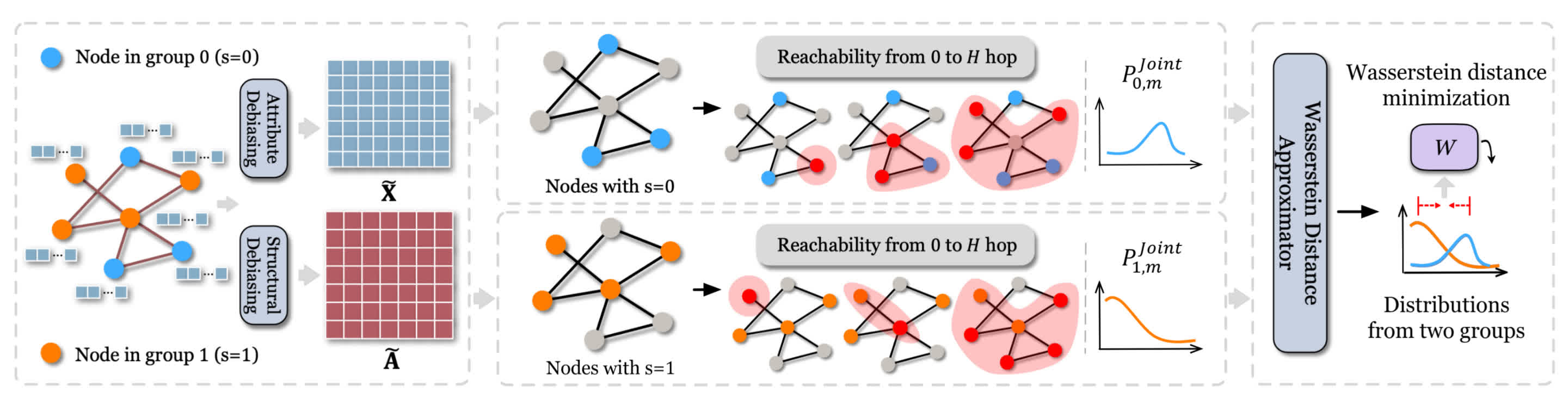

Objective optimizations

To transform the problem into a tractable, and end-to-end gradient-based optimization problem, the authors use a min-max optimization game :

Instead of finding the infinimum of the objective function, the Wasserstein Distance Approximator (WDA) is computed as a neural network, with clipped weights to satisfy a Lipschitz constraint, which makes the problem tractable
The attribute debiasing module uses a linear function to re-weight the features, to reduce the bias while trying to preserve the original information
The structure debiasing module also tries to stick as close as possible to the original information, as well as enforcing that \(\tilde{A}\) is symmetric and sparse
The adjacency matrix \(\tilde{A}\) needs to remain symmetric and sparse
The framework trains the WDA via Stochastic Gradient Descent to compute the bias, and the Attribute and Structural modules via Proximal Gradient Descent to reduce the bias

Once the main optimization is finished, two final post-processing steps occur :

Attribute masking : It sets the \(z\) smallest weights in the attribute matrix to zero, to remove the most biased attribute channels
Adjacency matrix binarization : A numerical threshold \(r\) is used to convert the continuous values of the adjacency matrix into a binary graph

Evaluation

The authors claim the hyper-parameters are tuned only based on their proposed bias metrics. They point out that the debiasing performance generalizes better, but is more difficult to tune.

They use a downstream task of node classification, with real-world and synthetic datasets :

Pokec-z and Pokec-n are collected from a Slovakian social network, a node is a user, an edge is a friendship relationship between users, the “region” is the sensitive attribute, and the task is to predict the working field of a user
UCSD34 is a facebook friendship network constructed similarly, here “gender” is the sensitive attribute, and the task is to predict whether a user belongs to a specific major
German credit represents a network of clients in a German bank, with edges formed between clients that have similar credit accounts, “gender” is the sensitive attribute, and the task is to classify the credit risk of clients
Recidivism is a graph representing defendants released on bail, connected with each other when they have similar past criminal record and demographics, the sensitive attribute being “race”, and the task is to classify the defendants in bail vs. no bail
in Credit Defaulter nodes are credit card users, and they are connected based on pattern similarity of their payments, “age” is the sensitive attribute, and the task is to predict whether a user will default on credit card payment.
The two synthetic datasets are based on the ones used in the introduction, with added attribute dimensions with gaussian noise, on an arbitrary classification task based on the random attributes

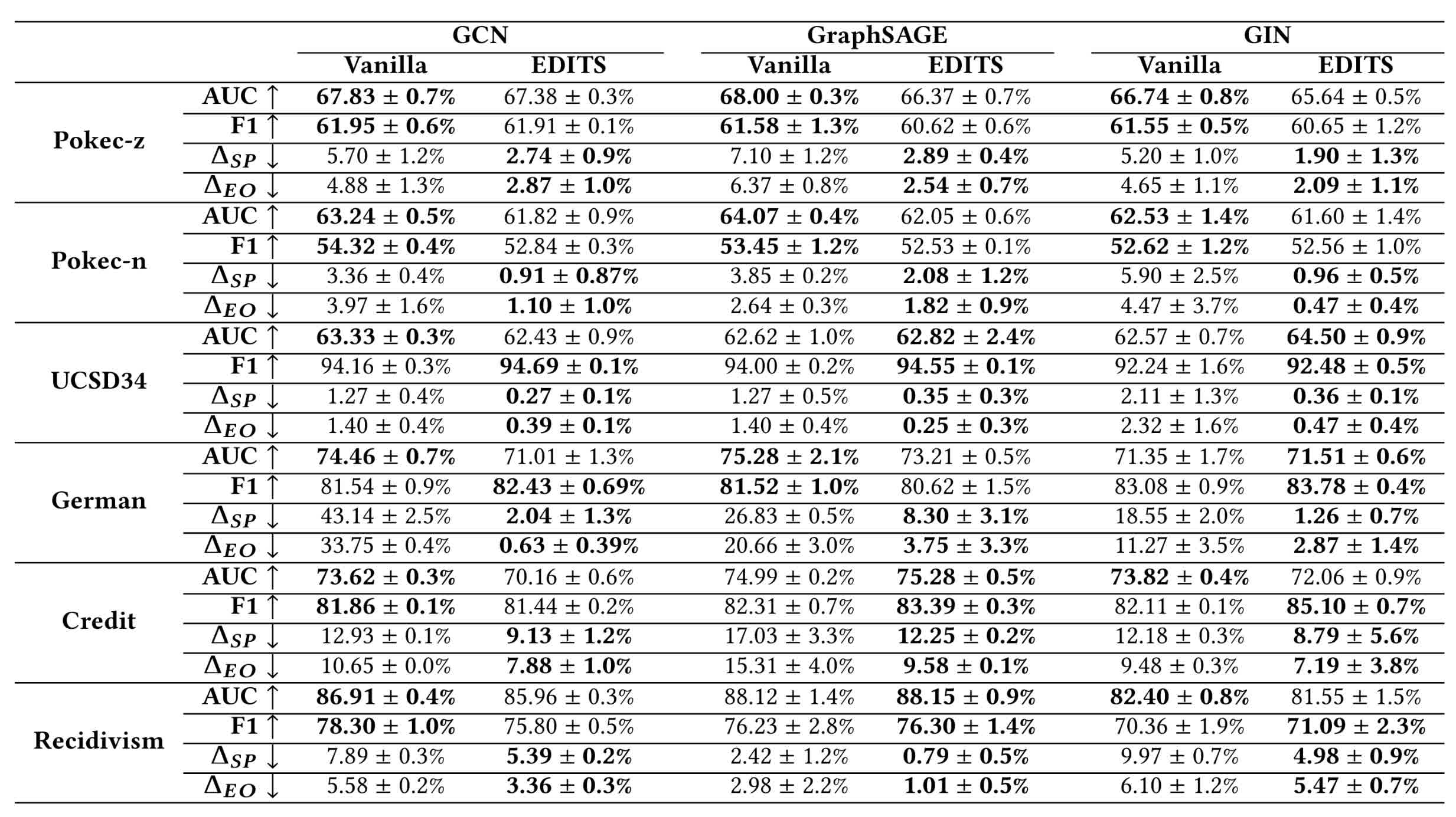
Regarding the fairness evaluation metrics, the authors use two common metrics to evaluate statistical parity and equal opportunity, evaluated on the test set (the lower the better) :

\[\Delta_{SP} = |P(\hat{y}=1|s=0) - P(\hat{y}=1|s=1)|\] \[\Delta_{EO} = |P(\hat{y}=1|y=1,s=0) - P(\hat{y}=1|y=1,s=1)|\]

where \(y\) denotes the label of a node, \(\hat{y}\) the prediction of a node label, and \(s\) the sensitive attribute.

Comparison with “baseline” methods (this is the first model-agnostic method):

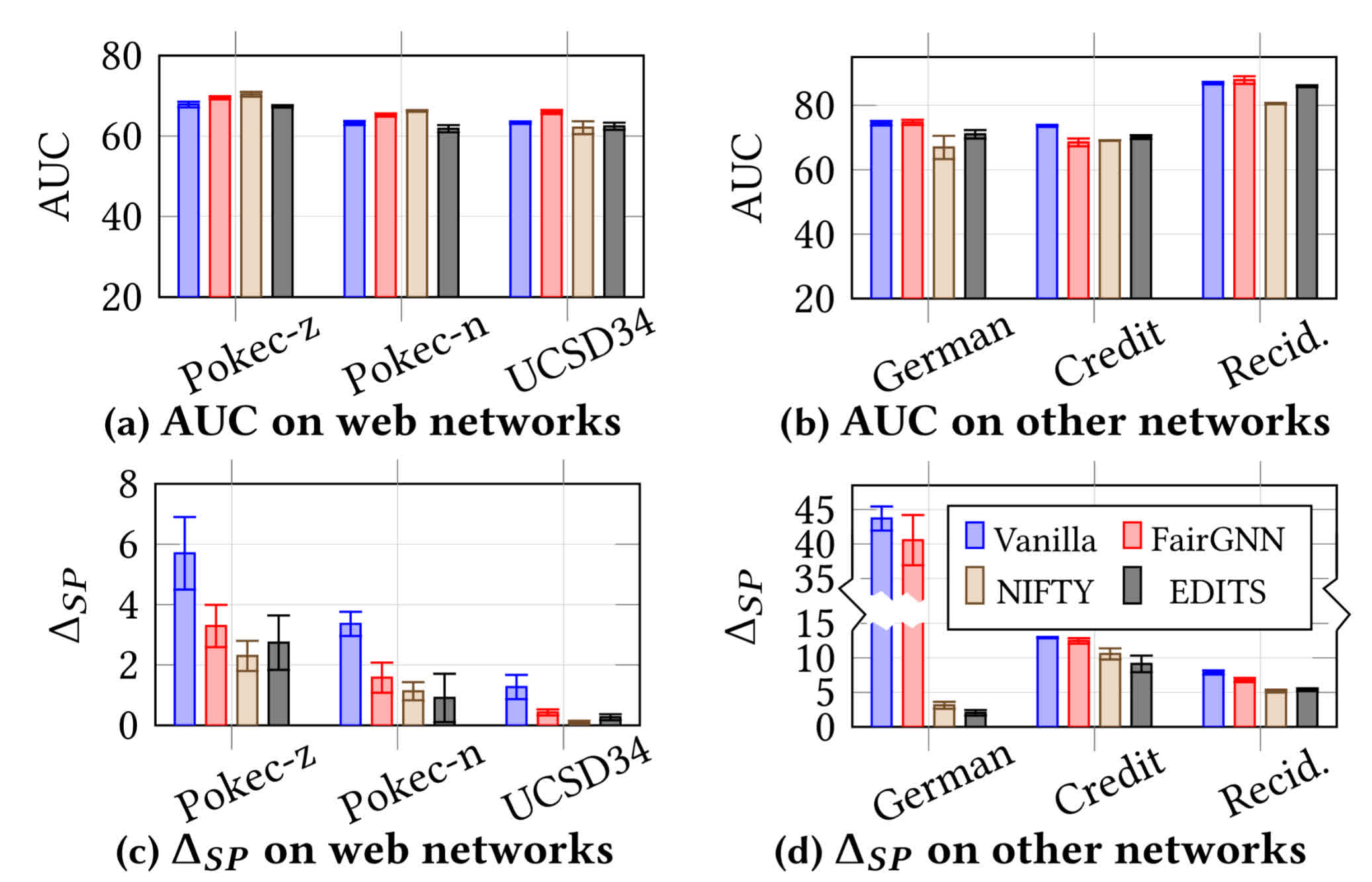
Utility and bias mitigation metrics on all the datasets :

Ablation study

Ablation of the attribute debiasing module and the structure debiasing module :

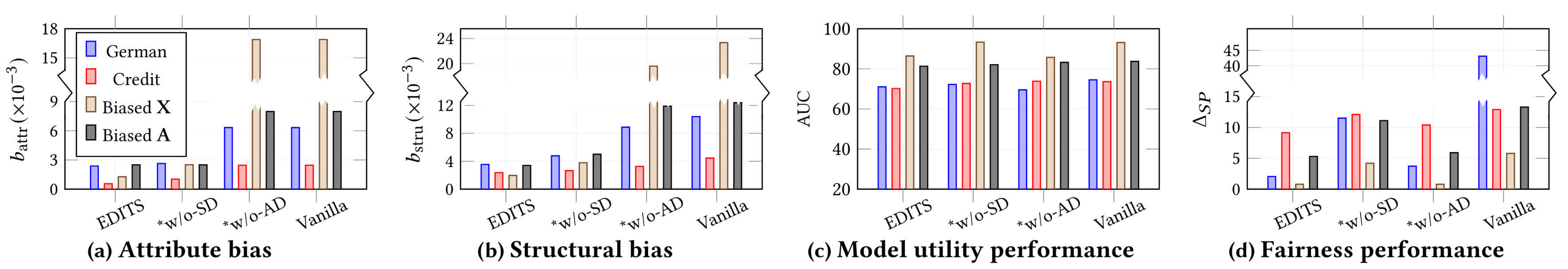
The ablation study involves removing one of the two bias correction modules (called “without structural bias correction” (w/o-SD) or “without attributive bias correction” (w/o-AD)). It shows that both modules contribute to reducing attributive and structural biases, with the reduction being much greater with the attributive bias correction module.

The effects of the individual modules also depend heavily on the dataset.

However, the authors emphasize that the structural bias removal module is essential for improving fairness performance (reduction in \(\Delta_{SP}\)).

Conclusion

This paper highlights the importance of combining both attribute and structure debiasing for graph datasets
The authors introduce the first model-agnostic debiasing method, based on the minimization of the Wasserstein distance between the debiased attribute distributions before and after the propagation, reaching SOTA performances
The framework has a lot of hyper-parameters, but its debiasing power generalizes better to the different datasets and GNN