Introduction to Score-based models
Notes
- This tutorial was inspired by this video tutorial and this post (both by the main author itself !)
- This other complete video tutorial may also help for comprehension
- Looking at this GitHub repo can give a quite simple and structured overview on how score-based models can be implemented.
Summary
- Introduction
- Score-based models
- Denoising score matching
- Quick reminder on diffusion models
- Stochastic differential equation (SDE)
- To go further : Conditional image generation and other examples
- References
Introduction
The main existing generative models can be divided in two categories :
- likelihood-based models, which goal is to learn directly the probability density function. Examples of these models are autoregressive models, normalizing flow or variational auto-encoders.
- implicit generative models, for which the density distribution is implicitly learnt by the model during sampling process. This is typically GANs, which have dominated the field of image generation during several years.
Such models each have their specific limitations. Likelihood-based models either have strong restrictions on the model architecture to make sure the normalizing constant of the distribution is tractable and VAEs rely on a substitutes of the likelihood the training. GANs have been historically the state-of-the-art of deep learning generative models in terms of visual quality but they do not allow density estimation and rely on adversarial learning, which is known to be particularly unstable.
In 2019 1 2, Yang Song proposed a paradigm for image generation based on the score function. Instead of trying to explicitly learn a density function, it aims to represent a data distribution by learning the gradient of the logarithm of the probability function .
Score-based models
Score matching
Suppose that we have training data \(\{x_1, x_2, ..., x_N\}\) that are supposed to be drawn from a distribution \(p(x)\). The goal is to find a \(\theta\)-parametrized density function \(p_{\theta}(x)\) that accurately estimate the real data density function. Without loss of generalization, we can write :
\[p_{\theta}(x) = \frac{e^{f_{\theta}(x)}}{Z_{\theta}}\]where \(Z_{\theta}\) is a such that \(\int p_{\theta}(x)dx = 1\). We would like to maximize the log-likelihood
\[\max_{\theta} \sum_{i=1}^{N} \log{p_{\theta}(x_i)}\]However, it requires \(p_{\theta}\) to be a normalized probability density function, which is in practice impossible for any general \(f_\theta\) as it means we have to evaluate \(Z_{\theta}\). The maximiziation of the log-likelihood is thus usually done by restricting the form of \(f_{\theta}\) (normalizing flow) or via a the expression of a lower bound (VAEs).
The idea behind the score-based models is to learn the gradients of the logarithm density function instead of the density function instead 3. This means that we are interested in approximating the quantity \(\nabla_x \log{p_{\theta}(x)}\), also called the score function. Indeed, we have :
\[\nabla_x \log{p_{\theta}(x)} = \nabla_x (\log{(\frac{e^{f_{\theta}(x)}}{Z_{\theta}})}) = \nabla_x f_{\theta}(x) - \underbrace{\nabla_x \log{Z_{\theta}}}_{=0} = \nabla_x f_{\theta}(x)\]so we don’t need to know the normalizing constant anymore. The goal of these models is hence to approximate this quantity by a network-parameterized function \(s_{\theta}(x) \approx \nabla_x f(x)\).
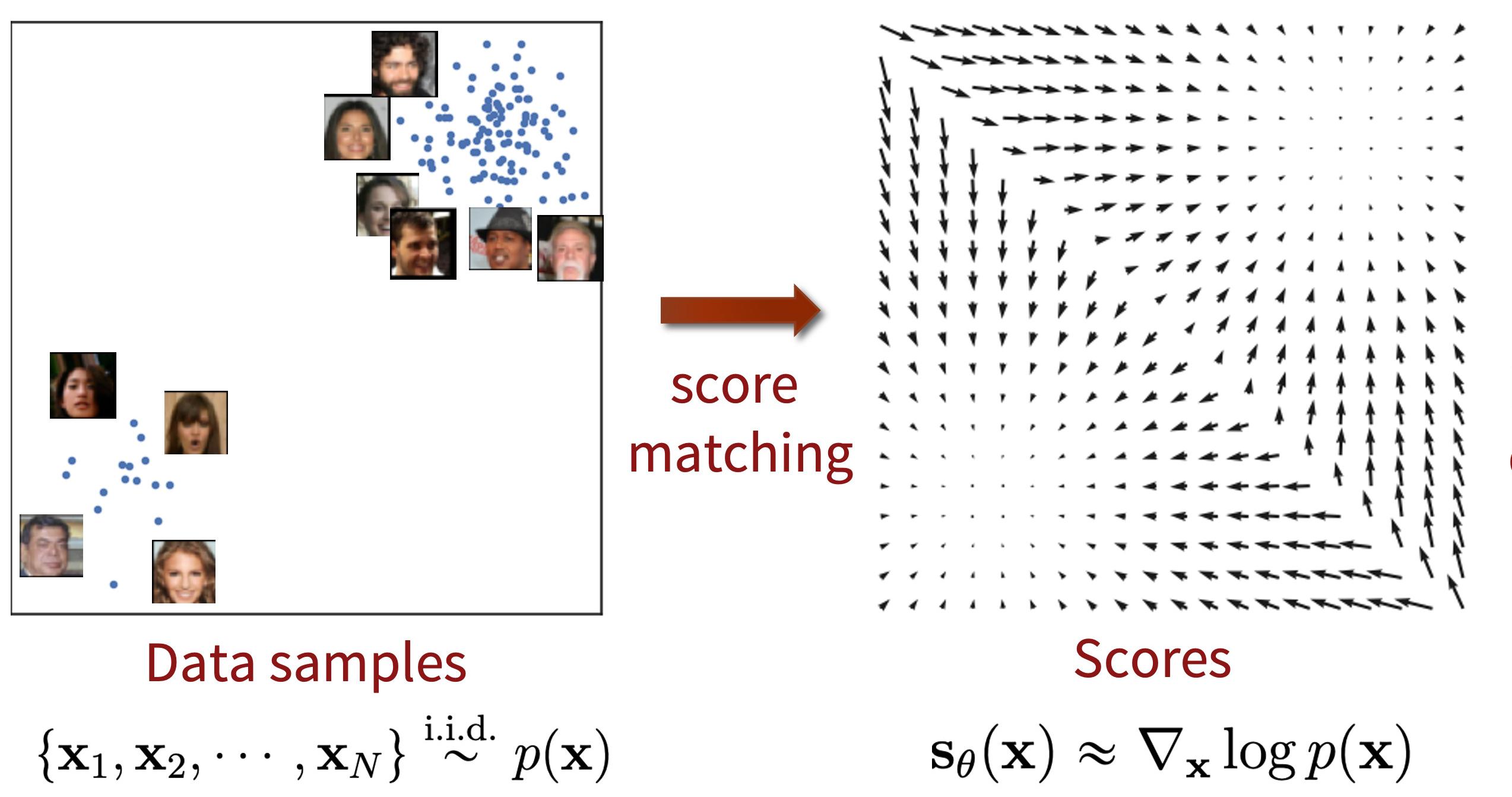
Figure 1. Illustration of score function estimation.
The optimization can be done via Fisher divergence :
\[\mathbb{E}_{p(x)} [\lVert \nabla_x \log{p(x)} - s_{\theta}(x) \rVert^2_2] \qquad (1)\]
Sampling with Langevin Dynamics
This paradigm of trying to approximate the score function of a density is motivated by the existence of a method that allows to sample data from a distribution if we know its gradients. Suppose we have a score-based model \(s_{\theta}(x) \approx \nabla_x \log{p(x)}\), we can use Langevin dynamics to draw samples from it. The principle is to follow a Monte Carlo Markov Chain, initialized at an arbitrary prior distribution \(x_0 \approx \pi(x)\) (usually a standard Gaussian distribution) and iterates as follows :
\[x_{i+1} = x_i + \epsilon \nabla_x \log{p(x)} + \sqrt{2 \epsilon} z_i , \qquad i=0,1, ..., K\]where \(z \sim \mathcal{N}(0,1)\). When \(\epsilon \to 0\) and \(K \to \infty\), the final \(x_K\) converges to a sample drawn of \(p(x)\). Hence having an approximation \(s_{\theta}(x)\) to plug is the previous equation above allow sampling from the score function.

Figure 2. Sampling with Langevin dynamics.
At this point, there is still a major issue : in equation (1), \(\nabla_x \log{p(x)}\) is intractable since it is linked to the data distribution that we aim to model.
A method to resolve this problem is to do sliced score matching 4. It uses a trick to rewrite (1) the expectation of a term that only depend on \(s_{\theta}(x)\) and its Jacobian plus a constant. Then, it uses projection towards random directions to make the approximation of the expectation computationnally tractable.
However, even if this method works theoretically, in practice, a score-based model trained as such as it will not produce new realistic samples, as shown in the figure below.
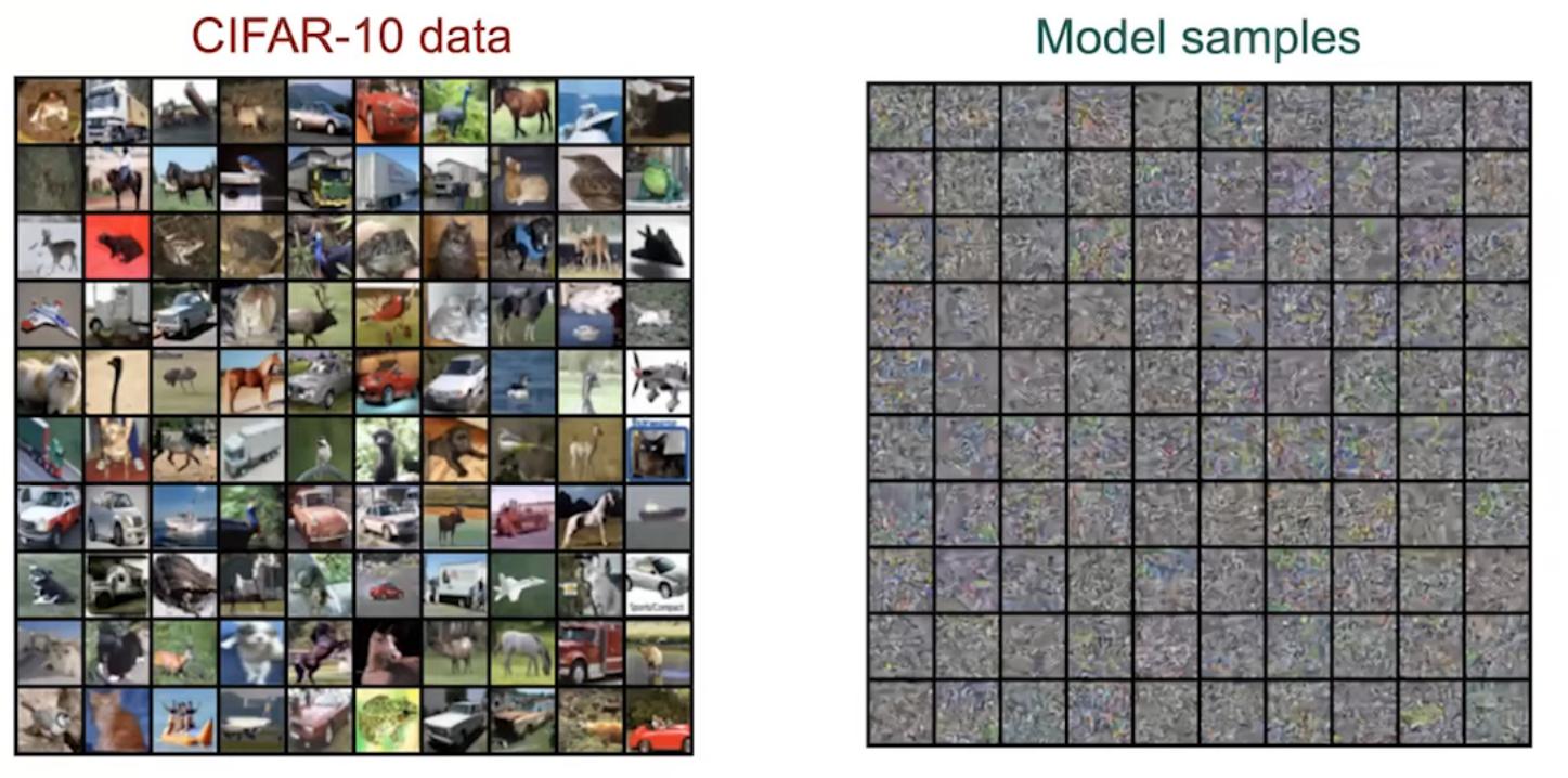
Figure 3. Example of image generated with a score-based model trained on CIFAR-10 with sliced score matching.
This is due to the fact that the model is only able to predict a good approximation of the score function in the regions where there is data. The estimated score functions are inaccurate in low density regions, where few data points are available to compute and optimize the score function.
\[\mathbb{E}_{p(x)} [\lVert \nabla_x \log{p(x)} - s_{\theta}(x) \rVert^2_2] = \int \textbf{p(x)} \lVert \nabla_x \log{p(x)} - s_\theta(x) \rVert_2^2dx\]
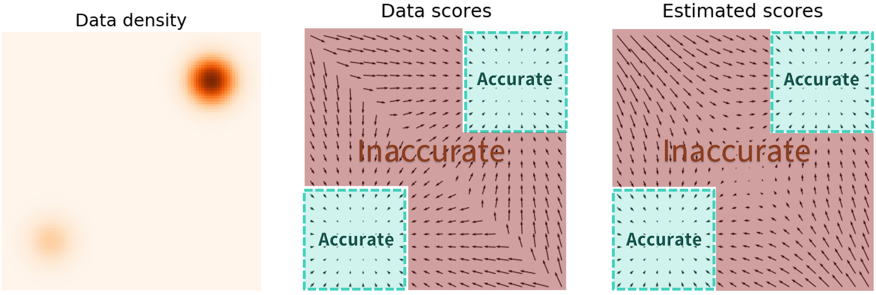
Figure 4. Data scores are poorly estimated in low data density regions.
A method called denoising score matching introduced in (Vincent, 2011) 5 allow both to bypass the formulation of the equation (1) and to get around the problem of the bad approximiation in low data density regions.
Denoising score matching
Principle
The main idea is to perturb the data density with a known noise (typically Gaussian) and use this new noisy distribution for the score function estimation. Let’s corrupt the data distribution \(p(x)\) with a Gaussian noise \(\mathcal{N}(0,\sigma^2)\); it gives the following noise-perturbed distribution :
\[p_\sigma(\tilde{x}) = \int p(x)\mathcal{N}(\tilde{x};x,\sigma^2I)dx\]It is very easy to sample data from \(p_\sigma(x)\) as it only requires to draw \(x\sim p(x)\) and compute \(x+\sigma z\) with \(z\sim \mathcal{N}(0,I)\).
Crucially, it has been shown that matching the scores of \(p_\sigma (x)\) as in (1) is equivalent to minimising the following objective function :
\[\mathbb{E}_{x \sim p(x)} \mathbb{E}_{\tilde{x}\sim p_\sigma(\tilde{x} \vert x)} \left[ \lVert s_\theta(\tilde{x}) - \nabla_{\tilde{x}}\log(p_\sigma (\tilde{x} \vert x)) \rVert _2^2 \right]\]What is good with the formula is that the conditional probability density function is analytically known so we can easily compute \(\nabla_{\tilde{x}}\log(p_\sigma (\tilde{x} \vert x)) \propto - \frac{\tilde{x} - x}{\sigma^2}\), which allow for direct optimization of the objective function.
The noisy distribution introduces a trade-off between matching with the data and exploration of the space. Indeed, high noise provides useful information for Langevin dynamics (exploration of low data density regions), but a density that is too disturbed no longer approximate the true data repartition. The solution is to consider a family of increasing noise levels \(\sigma_1 < \sigma_2 < ... < \sigma_L\) such that \(p_{\sigma_1}(x) \approx p(x)\) and \(p_{\sigma_L}(x) \approx \mathcal{N}(0,1)\) and to train a noise conditional score-based model \(s_{\theta}(x, \sigma_i)\) with score matching such that \(s_{\theta}(x,\sigma_i) \approx \nabla_x p_{\sigma_i}(x)\) for all \(i=1,2,...,L\).
The new training objective is a weighted sum of Fisher divergences for all noise scales :
\[\sum_{i=1}^{L} \lambda (i) \mathbb{E}_{x \sim p(x)} \mathbb{E}_{\tilde{x}\sim p_\sigma(\tilde{x} \vert x)} \left[ \left\Vert \sigma_i s_{\theta}(x,\sigma_i) + \frac{\tilde{x} - x}{\sigma_i} \right\Vert _2^2 \right]\]With this new way of doing, a T-step Langevin dynamics sampling is decomposed in L consecutive substeps of \(T/L\) iterations performed with decreasing noise scaling (i.e. from \(i=L\) to \(i=1\)). This is called annealed Langevin dynamics (Fig. 5, sampling step are illustrated from right to left).
Figure 5. Annealed Langevin Dynamics.
Examples of results
In 2021, a score-based model established new state-of-the-art performances for image generation on CIFAR-10 with an Inception score of 9.89 and FID of 2.20, beating previous best model StyleGAN2-ADA.
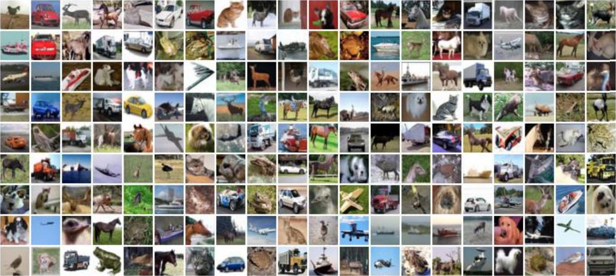
Figure 6. Example of image generated with a score-based model trained on CIFAR-10.
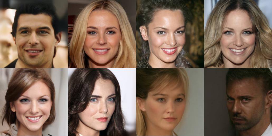
Figure 7. Examples of samples generated from a score-based model trained on CelebA-HQ (1024x1024).
Quick reminder on diffusion models
A diffusion model 6 7 8 consists in converting from a known, simple and tractable distribution \(\pi(x)\) (typically a standard Gaussian) to a target distribution \(p_{data}(x)\) using a Markov chain.
The forward process consists in corrupting an input image \(x_0\) via a T-step Markov chain where at each step, a small amount of noise is added to the image. Given an image \(x_t\) at time step \(t\), we produce the next image with a Gaussiance noise with variance \(\beta_t\) :
\[q(x_{t+1}|x_t)=\mathcal{N}(x_{t+1}, \mu_t = \sqrt{1-\beta_t}x_t, \Sigma_t = \beta_t \textbf{I})\]More practically, a ‘slightly more noisy image’ is generated (at a pixel level) via :
\[x_{t+1} = \sqrt{1-\beta_t}x_t + \sqrt{\beta_t}\epsilon\]with \(\epsilon \sim \mathcal{N}(0,1)\)
The total number of diffusion steps T, as well as the noising schedule \(\beta_t\) must be specified. T is typically of several thousands and \(\beta_t\) variates linearly from \(\beta_1 = 10^{-4}\) to \(\beta_T = 0.02\) in CITER DDPM, even though other schedule have proven to be more efficient since then.
A nice reperametrization trick makes it easier to generate a sample \(x_t\) in a non-recursive manner, allowing to generate at any time point \(t\) from a data point \(x_0\). Indeed, define \(\alpha_t = 1 - \beta_t\) and \(\overline{\alpha_t} = \prod_{s=0}^{t} \alpha_s\), and take \(\epsilon_0,..., \epsilon_{t-1} \sim \mathcal{N}(0,\textbf{I})\), we have:
\[\begin{aligned} x_t &= \sqrt{1-\beta_t}x_{t-1} + \sqrt{\beta_t}\epsilon_{t-1} \\ & = \sqrt{\alpha_t} x_{t-2} + \sqrt{1-\alpha_t}\epsilon_{t-2} \\ & = \; ... \\ & = \sqrt{\overline{\alpha_t}}x_0 + \sqrt{1 - \overline{\alpha_t}}\epsilon_0 \end{aligned}\]Thus, to produce a sample \(x_t\) from \(x_0\), one can simply use the following distribution :
\[x_t \sim q(x_t|x_0) = \mathcal{N}(x_t; \sqrt{\overline{\alpha_t}} x_0, (1-\overline{\alpha_t})\textbf{I})\]
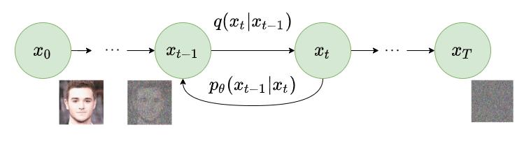
Figure 8. Forward and reverse diffusion process.
With the diffusion process that we have just described, when \(T \to \infty\), the corrupted \(x_T\) are nearly drawn from an isotropic Gaussian distribution. The goal is to learn the reverse diffusion process, i.e. to learn te \(q(x_{t-1} \vert x_t)\), in order to be able to generate new data samples from pure Gaussian noise. In practical, the reverse distribution can not be computed analitically, so we’d like to train a model with parameters \(\theta\) such that for any time step \(t\) :
\[p_{\theta}(x_{t-1}|x_t) := \mathcal{N}(x_{t-1}; \mu_\theta(x_t, t), \tilde{\beta}_t\textbf{I}) \approx q(x_{t-1}|x_t)\]For training, the negative log-likelihood is limited by an upper bound wich allows to train the model thanks to :
\[\mathbb{E}_{t\sim [0,...,T], x_0 \sim p(x), x_t \sim q(x_t \vert x_0) } \left[ \left\Vert \tilde{\mu}_t(x_t, x_0) - \mu_\theta (x_t,t) \right\Vert_2^2 \right]\]with \(\tilde{\mu}_t = \frac{1}{\sqrt{\alpha_t}}(x_t - \frac{1 - \alpha_t}{\sqrt{1-\overline{\alpha}_t}}\epsilon_t)\)
In practice, instead of trying to learn to reconstruct \(x_{t-1}\) from \(x_t\), we will train a model to learn \(\epsilon_\theta(x_t,t)\), that is to say the noise that was generated to generate \(x_{t}\) from \(x_0\), with the following loss :
\[\mathbb{E}_{t\sim [0,...,T], x_0 \sim p(x), \epsilon \sim \mathcal{N}(0,1)} \left[ \lambda_t \lVert \epsilon - \epsilon_\theta (\underbrace{\sqrt{\overline{\alpha}_t}x_0 + \sqrt{1 - \overline{\alpha}_t}\epsilon}_{x_t}, t) \rVert_2^2 \right]\]
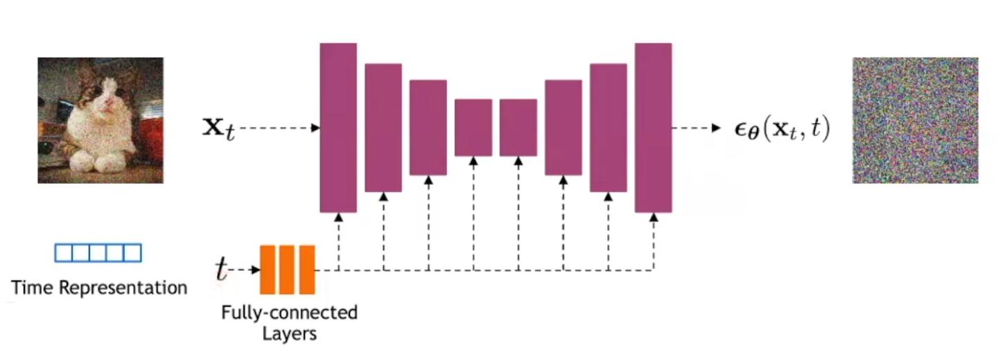
Figure 9. Illustration of how a neural network can be trained as a diffusion model. We typically use a UNet-like model where all the stages are conditioned by the time step.
To summarize, a diffusion model will be trained and then able to generate new data samples thanks to the two following algorithmic processes :

Figure 10. Pseudo-code for training and sampling of diffusion models.
Stochastic differential equation (SDE)
In the previous sections, we introduced two discrete stochastic processes where an image is corrupred by a gradually increasing noise. When the number of noise scales approaches infinity, they become continuous-time stochastic processes.

Figure 11. From discrete to continuous stochastic probabilistic process.
A stochastic process \(\{ \text{x} \}_{t \in [0,T]}\) is an infinite ensemble of random variables associated with their probability densities \(\{ p_t(\text{x}) \} _{t \in [0,T]}\). Many stochastic processes, incuding diffusion can be described by a stochastic differential equation (SDE) :
\[d\text{x}_t = f(\text{x}_t, t)dt + \sigma(t)dw_t\]where \(f(\cdot, t) : \mathbb{R}^d \to \mathbb{R}^d\) is a deterministic drift, \(\sigma(t) \in \mathbb{R}\) is the diffusion coefficient and \(w_t\) the standard Brownian motion, whose infinitesimal variation \(d_w\) can be seen as white noise and discretized \(dw_{\epsilon} = \sqrt{\epsilon} \mathcal{N}(0,1).\)
A SDE can be reversed using the score function thanks to the following formula :
\[dx = [f(\text{x},t) - \sigma(t)^2 \nabla_x \log{p_t(\text{x})} ]dt + \sigma(t) d\overline{w}\]where \(d\overline{w}\) is the Brownian process when time flow backwards from 0 to T and \(dt\) is an negative timestep. Here again, it is possible to generate sample once the score of each marginal distribution \(\nabla_x \log{p_t(x)}\) is well approximated by a time dependant model \(s_{\theta} (x,t)\). In practice, a sample x is obtained by solving the previous SDE using Euler-Maruyama method, which is the equivalent of Euler method for ODEs.
Figure 12. Illustration of the reverse SDE process.
In a similar manner to the discrete case seen before, such a model is optimized though the objective function :
\[\mathbb{E}_{t \sim Uniform[0,T], x_0, x(t)} \left[ \lambda (t) \lVert \nabla_{x(t)} \log{p(x(t) \vert x(0))} - s_{\theta}(x(t),t) \rVert_2^2 \right]\]
Link with Score-based Models with Langevin Dynamics (SMLD) and Denoising Diffusion Probabilistic Models (DDPM)
Both Score-based models with Langevin dynamics et Denoising diffusion probabilistic models are essentially particular cases of a stochastic differential equation.
Indeed, DDPM, first introduced as a process described by a Markov chain, can also be seen as a discretization of a SDE :
\[\begin{align} \text{Markov chain} & \qquad x_i = \sqrt{1 - \beta _i} \text{x}_{i-1} + \sqrt{\beta _i}\text{z}_{i-1}\\ SDE & \qquad d\text{x} = -\frac{1}{2} \beta (t) \text{x} \, dt + \sqrt{\beta(t)} dw \end{align}\]Similarily, a SMLD process described earlier with a sequence of increasing noise level \(\sigma_1 < \sigma_2 < ... < \sigma_L\) has the same two possible interpretations :
\[\begin{align} \text{Markov chain} & \qquad x_i = x_{i-1} + \sqrt{\sigma^2_i - \sigma^2_{i-1}}\text{z}_{i-1}\\ \text{SDE} & \qquad d\text{x} = \sqrt{\frac{\text{d}[\sigma^2(t)]}{\text{d}t}} dw \end{align}\]Score-based models and DDPM are thus almost equivalent as they are a discretization of the same continuous stochastic process. The main difference is that the SDE which DDPM are derived from is Variance Preserving while the one from which SMLD comes from is Variance Exploding. Since then, other SDEs have proven to give better results in terms of computational stability and performances for data generation and density estimation.
Note also that the noise \(\epsilon_\theta(x_t,t)\) that diffusion models aim to estimate is linked to the score function : \(s_\theta(x_t,t) = - \frac{\epsilon_\theta(x_t,t)}{\sigma(t)}\)
Probability flow ODE and density estimation
A Stochastic Differential Equation have an associated non-stochastic ordinary differential equation, called probability flow ODE, such that their trajectories have the same marginal probability density \(p_t(x)\) :
\[d\text{x} = \left[ f(\text{x},t) - \frac{1}{2}\sigma(t)^2 \nabla_x \log{p_t(\text{x})} \right]dt\]
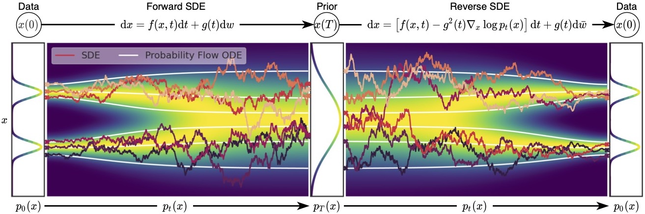
Figure 13. A SDE have an associated probabilistic flow ODE (white lines), that is not stochastic. Both reverser SDE and probability flow ODE can be obtained by estimating score functions
A useful application of such a transform is to allow exact log-likelihood computaion, levaring change-of-variable for ODEs (here written to simplify in the case where \(f(x,t)=0\)):
\[\log{p_\theta} = \log{\pi(\text{x}_T}) - \frac{1}{2} \int_0^T \sigma(t) \text{trace}(\nabla_x s_\theta (\text{x}, t))dt\]Note that \(\text{trace}(\nabla_x s_\theta (\text{x}, t))\) is not easy to compute but it can be approximated by a non-biased stochastic estimator called Skilling-Hutchinson estimator
Probability flow ODEs can also benefit from fast ODE solvers and allow image interpolation in the latent space with semantic coherence in the image domain.
Such models acheived state-of-the-art log-likelihood estimation on CIFAR-10, surpassing normalizing flow and other models.

Figure 14. NLL and FID of diffusion models on CIFAR-10.
To go further : Conditional generation and other examples
All the methods described above quite easily extend to conditional generative tasks. In that case, the obkective is the train a model to match the score function \(\nabla_x p(x \vert y)\) where \(x\) are samples from data distribution and \(y\) is conditional information associated with each sample.
Approaching this task though score estimation as it is done with SMLD exhibits a nice trick. Indeed, leveraging Bayes’ rule, we have :
\[p(\text{x} \vert \text{y}) = \frac{p(\text{x})p(\text{y} \vert \text{x})}{p(\text{y})}\]\(p(\text{y})\) is unknown but this expression simplify when using the gradients with respect to \(x\) :
\[\nabla_x \log{p(\text{x} \vert \text{y})} = \nabla_x \log{p(\text{x})} + \nabla_x \log{p(\text{y} \vert \text{x})} - \underbrace{\nabla_x \log{p(\text{y}})}_{=0}\]Hence, it is possible to approximate the conditional score funtion by training first a model to predict the unconditional data distribution \(s_{\theta}(x)\), and in a second step the conditioned score function \(\nabla_x \log{p(\text{x} \vert \text{y})}\).
More examples of results
Many problems can be formulated as conditional generation such as image inpainting, colorization, super-resolution, solving inverse problems and many other. In this section we show examples of results that can be obtained with conditional score-based model, as well as other applications in which diffusion/score-based models have already been applied 2 9 10 11 12.

Figure 15. Conditional score-based model for image inpainting.

Figure 16. Conditional score-based model for image colorization.

Figure 17. Diffusion model for text-conditioned image generation.

Figure 18. Conditional score-based model for CT-scan reconstruction with 23 projections.

Figure 19. Diffusion model for 3D shape generation.
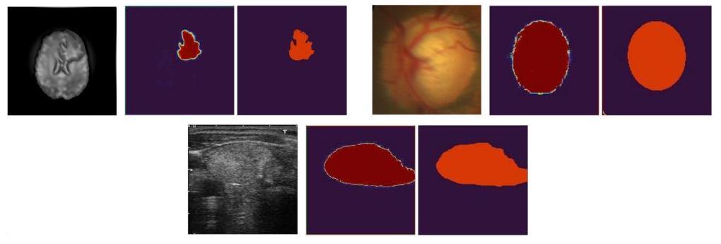
Figure 20. Image-conditioned diffusion model medical image segmentation.
References
-
Y. Song, S. Ermon Generative Modeling by Estimating Gradients of the Data Distribution, 2019 ↩
-
Y. Song, J. Sohl-Dickstein, D. P. Kingma, A. Kumar, S. Ermon, B. Poole Score-Based Generative Modeling through Stochastic Differential Equations, 2020. ↩ ↩2
-
A. Hyvärinen Estimation of non-normalized statistical models by score matching, 2005. ↩
-
Y. Song, S. Garg, J. Shi, and S. Ermon Sliced score matching: A scalable approach to density and score estimation, 2019. ↩
-
P. Vincent A connection between score matching and denoising autoencoders, 2011. ↩
-
J. Sohl-Dickstein, E. Weiss, N. Maheswaranathan, S. Ganguli Deep unsupervised learning using nonequilibrium thermodynamics, 2015. ↩
-
J. Ho, A. Jain, P. Abbeel Denoising Diffusion Probabilistic Models, 2020. ↩
-
L. Yang, Z. Zhang, Y. Song, S. Hong, R. Xu, Y. Zhao, W. Zhang, B. Cui, MN-H. Yang Diffusion Models: A Comprehensive Survey of Methods and Applications, 2022. ↩
-
R. Rombach, A. Blattmann, D. Lorenz, P. Esser, B. Ommer High-Resolution Image Synthesis with Latent Diffusion Models ↩
-
Y. Song, L. Shen, L. Xing, S. Ermon Solving Inverse Problems in Medical Imaging with Score-Based Generative Models, 2022. ↩
-
X. Zeng, A. Vahdat, F. Williams, Z. Gojci, O. Litany, S. Fidler, K. Kreis LION: Latent Point Diffusion Models for 3D Shape Generation, 2022. ↩
-
J. Wu, R. Fu, H. Fang, Y. Zhang, Y. Yang, H. Xiong, H. Liu, Y. Xu MedSegDiff: Medical Image Segmentation with Diffusion Probabilistic Model, 2022. ↩