Introduction to Flow Matching
Note
The aim of this tutorial is to present general concepts and fundamentals about flow matching, introduced from the point of view of normalizing flows.
The following ressources can be useful for those who would like to delve deeper into this topic (most of the illustrations shown in the post are taken from these sources) :
- Y. Lipman et al., Flow Matching Guide and Code, arxiv link.
- R. T. Q. Chen et al., Flow Matching for Generative Modeling, NeurIPS 2024 Tutorial link.
- T. Fjelde et al., An introduction to Flow Matching, Cambridge MLG Blog, link.
- A. Gagneux et al., A Visual Dive into Conditional Flow Matching, ICLR Blogposts 2025, link.
Summary
- Note
- Summary
- From Normalizing Flows to Flow Matching
- Deep dive into Flow Matching
- Link with SDE, ODE and Diffusion Models
- To go further : advanced concepts
- Conclusion
- References
From Normalizing Flows to Flow Matching
Reminder on Normalizing Flows
As our goal is to present Flow Matching from the starting point of view of Normalizing Flows, this section is a an introduction to this type of models. They can be used for data generation, and will be presented from this viewpoint. For a more complete presentation of Normalizing Flows, please refer to this tutorial.
Let \(x \in X\) be a random variable with a density function \(p_{X}\) and denote \(f : X \to Z\) a diffeomorphism. The change of variable operated by \(f\) can be used to transform \(x \sim p_{X}(x)\) into a simpler random variable \(z = f(x)\), with \(z \sim p_{Z}(z)\). One probability density can be retrieved from the other with the following formula :
\[p_{X}(x) = p_{Z}(f(x)) |\text{det}( \frac{\partial f(x)}{\partial x})|\]where \(\frac{\partial f}{\partial z}\) is the Jacobian matrix of the application \(f\) and \(\text{det}(\cdot)\) designates the determinant of a matrix. Note that \(f\) is a diffeomorphism and thus this model can be done in the two directions, i.e. from a simple distribution to a complex one (data generation) or from a complex distribution to a simpler one (encoding).
Normalizing flow is a type of generative model that leverages the change-of-variables formula. We learn to transform a complex distribution into a simpler one (typically a multivariate normal distribution) though a serie of invertible mappings, then generation is done with the inverse transformation. Indeed, it is possible to stack in sequence several of the diffeomorphisms introduced above \(f_1, ..., f_K\):
\[f = f_K \circ f_{K-1} \circ \, ... \circ f_1\]During the successive modifications, a sample \(x\) from real data flows though a sequence of transformations and is progressively “normalized”. The following figure illustrates the principle of this type of model :
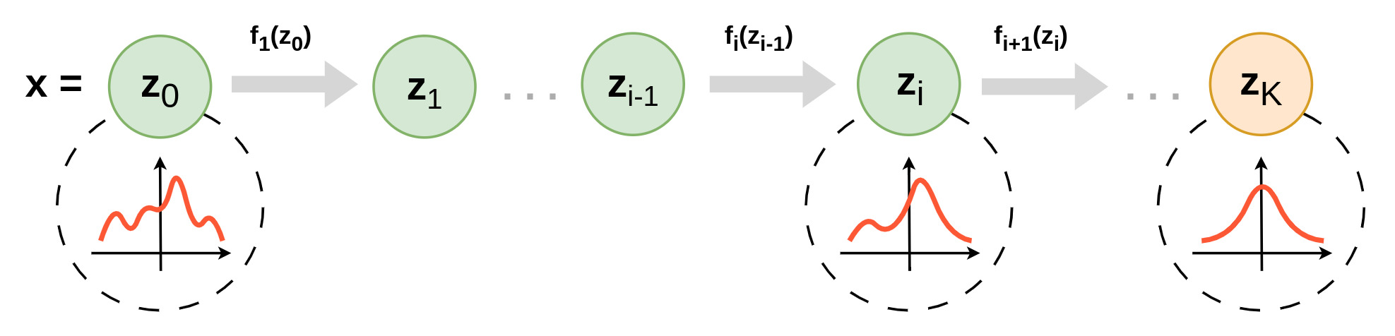
Figure 1. Illustration of a model of normalizing flow.
Given such transformation, it is possible to compute directly the likelihood of some data observed \(x = \{x^{(i)}\}_{i=1,...,N}\). This is an interesting property because it allows for parameter optimization through direct log-likelihood maximization, without relying on a lower bound of the likelihood, as is the case with VAEs for example. It is computed as follows :
\[\log p(x;\theta, \psi) = \sum_{i=1}^{N} \log p_{Z}(f(x^{(i)};\theta) ; \psi) + \log |\text{det} \frac{\partial f(x^{(i)};\theta)}{\partial x^{(i)}} | \\ = \sum_{i=1}^{N} \log p_{Z}(f(x^{(i)};\theta);\psi) + \sum_{k=1}^{K} \log |\text{det} \frac{\partial f_{k}(x_{k-1}^{(i)};\theta_k)}{\partial x_{k-1}^{(i)}} |\]where \(\theta=(\theta_1,...,\theta_K)\) and \(\psi\) respectiveley denotes the parameters of the transformation \(f\) and the target distribution \(p_{Z}\).
Theoretically, any diffeomorphism could be used to build a normalizing flow model, but in practice it should satisfy two properties to be applicable:
- Be invertible with an easy-to-compute inverse function
- Computing the determinant of its Jacobian needs to be efficient. Typically, we want the Jacobian to be a triangular matrix.
One of the earliest types of functions used in normalizing flows is the planar flow, which has the following form :
\[f(x) = x + a h(b^{T} x + c)\]where \(\lambda = \{a \in \mathbb{R}^{D}, b \in \mathbb{R}^{D}, c\in \mathbb{R} \}\) are free parameters and \(h(\cdot)\) is a differentiable element-wise and non-linear function.
Continuous Flow Matching
With normalizing flows, the types of transform that can be used is restricted and thus directly limits the expressivity of parametrized approximators. As mentioned above, a workaournd is to stack small, atomic transforms. Typical networks, such as FastFlow, designed for unsupervised anomaly detection, contains between 4 and 12 layers of such transforms.
An idea that naturally comes to mind when working with normalizing flows would be to increase the numbers of flows building blocks and increase their number to 100, 1000 or more. At the limit, we could even have an infinite number of such blocks. Obviously, in practice it is impossible to train that many blocks, but instead we could parametrize a build block by a time parameter \(t\) : \(f(x, t;\theta)\).
With such network – hypothetical for now –, a single forward pass would require to perform \(T=10, 100, 1000, ...\) passes through this small, infinitesimal building block.
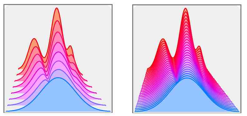
Figure 2. At the limit of stacking several normalizing flow blocks (left) we can imagine an infinitesimal, time-parametrized continuous normalizing flow (right). From [A.Gagneux et al.].
A similar idea also emerges if we take a look back at the expression of the planar flow. In the equation \(x_{k+1} := f_k (x_k) = x_k + a_k h(b_k^{T} x_k + c_k)\), if we let \(u_k (\cdot) \overset{def}{=} K a_k h(b_k^{T} \cdot + c_k)\) we can write :
\[x_{k+1} = f_k (x_k) = x_k + \frac{1}{K} u_k (x_k)\]This equation can be interpreted as an Euler step discretization of the following Ordinary Differential Equation (ODE) :
\[\begin{cases} x(0) = x_0 \\ \partial_t x(t) = u(x(t), t), \; \forall t \in [0,1] \end{cases}\]We thus found ourselves with an initial value problem controlled by \(u_{\theta} : \mathbb{R}^{d} \times [0,1] \rightarrow \mathbb{R}^d\), called the velocity field. We also introduce two very important terms :
- the flow \(f : \mathbb{R}^{d} \times [0,1] \rightarrow \mathbb{R}^d\) where \(f(x,t)\) is the solution to the initial value problem at time \(t\).
- the probability path \((p_t)_{t \in [0,1]}\), which is the distribution of \(f(x,t)\) when \(x \sim p_0\), i.e. the density when the intial data distribution follows the path described by the velocity field \(u_{\theta}\).
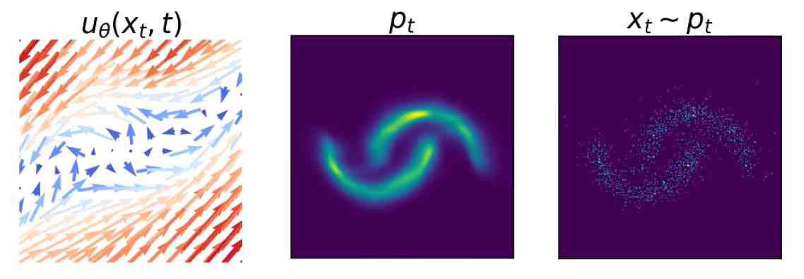
Figure 3. Generating a target distribution p1 from an initial distribution (typically a centered Gaussian distribution) consists in building a velocity field ut (left) which allows to create a continuous series of probability paths (center and right). From [A.Gagneux et al.].
To train the model, or at inference, it is possible to compute the exact likelihood of a data point \(x^{(i)}\) at time \(t\) with the formula :
\[\log p_t (x^{(i)}) = \log p_0 (x(0)) - \int_0^1 \nabla \cdot u_{\theta}(\cdot, \tau)(x(\tau)) d\tau\]Although very appealing at first sight, the Continuous Normaling Flow suffers from several limitations :
- the training procedure via log likelihood maximization with the formula above requires integrating the source distribution according to the velocity field. This approach is sometimes called with simulation, and it does not scale well is higher dimension, such as images.
- the learning process is not stable, likely because of numerical approximations or, more importantly, to the infinite number of possible probability paths (Figure 4)
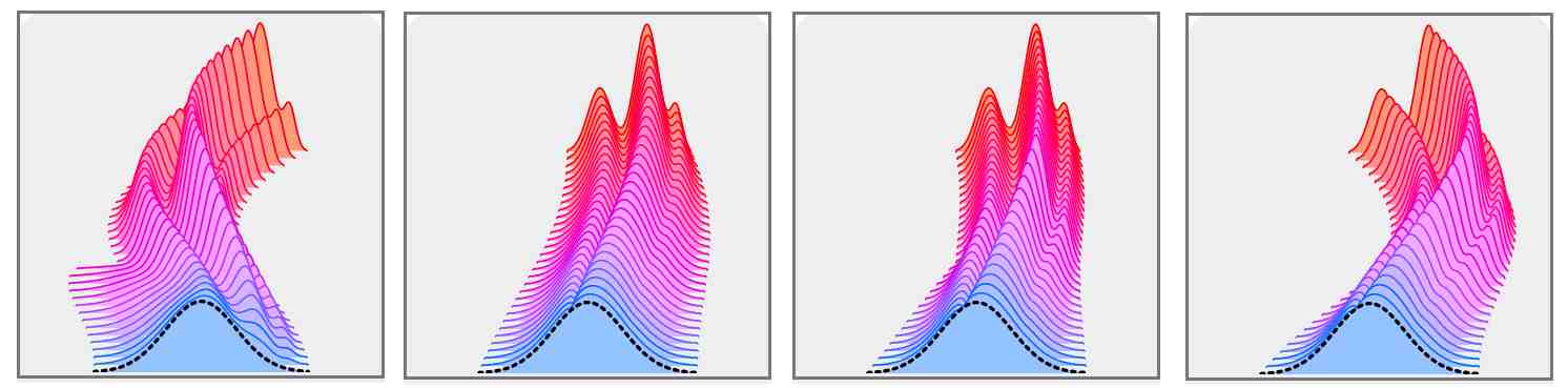
Figure 4. For given source and target distributions, there exists an infinite number of possible solutions of probability paths. From [A.Gagneux et al.].
Deep dive into Flow Matching
Conditional Flow Matching to solve the limits of Continuous Normalizing Flows
The idea behind Flow Matching is the same as Continuous Normalizing Flows, that is learning a velocity field \(u_{\theta}(x,t)\) such that, when followed, it transforms the source distribution \(p_0\) (typically centered Gaussian, but we will come back to that later) into the target distribution \(p_{\textrm{data}}\).
To set the problem more formally, let’s rename respectively these source and target random variables \(X_0\) and \(X_1\). We recall that we are looking for a vector field \(u : \mathbb{R}^D \times [0,1] \rightarrow \mathbb{R}^D\) which allows to go from \(X_0 \sim p\) to \(X_1 \sim q\) (or sometimes we will write \(p_{\textrm{data}}\) instead of \(q\)). In our case, the velocity field will be a \(\theta\)-parametrized neural network. This velocity field also defines a time-dependant flow \(\psi : \mathbb{R}^D \times [0,1] \rightarrow \mathbb{R}^D\) defined as :
\[\frac{\textrm{d} \psi_t (x)}{\textrm{d}t} = u_t (\psi_t (x))\]The goal of Flow Matching is hence to learn a vector field \(u_{\theta , t}\) such that its flow \(\psi_t\) is such that \(X_t \overset{def}{:=} \psi_t(X_0) \sim p_t \textrm{ for } X_0 \sim p_0\), i.e. it generates a probability path \(p_t\) with \(p(t=0) = p\) and \(p(t=1) =q\).
As explained before, there exists an infinite number of possible probability paths (and thus velocity fields) \(p_t\). We would like to specify in advance which probabilty path we want to estimate. However, since \(q\) (“\(p_{\textrm{data}}\)”) is not known, it is directly not possible to choose a probability path. The only things we can do is sample examples from this target distribution \(p_{\textrm{data}}\).
The solution proposed by the authors of the paper which originally introduced Flow Matching1 is to choose a probability path conditioned by the source and target distributions, i.e. we will learn \(p_t = p(x \mid t,x_0,x1)\).
Among all possible paths, we can choose to use the one that interpolates between the source and target distributions in straight line. . We define the time-dependant random variable :
\[X_t = tX_1 + (1 - t)X_0 \sim p_t\]It is straightfoward to verify that \(X_{t=0} = X_0\) and \(X_{t=1} = X_1\), and to compute how this choice of conditioned probability paths allows to easily compute the (true) vector field :
\[u_t = \frac{\textrm{d} \psi_t (x)}{\textrm{d}t} = X_1 - X_0\]Hence, we easily derive the Flow Matching Loss that will be used to train an approximation \(u_t^{\theta}\) of the velocity field :
\[\mathcal{L}_{\textrm{CFM}} (\theta) = \mathbb{E}_{t,X_0,X_1} \lVert u_t^{\theta} - \underbrace{(X_1 - X_0)}_{=u_t} \rVert ^2\]where \(t \sim U[0,1]\), \(X_0 \sim p\) and \(X_1 \sim q\)
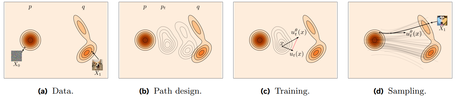
Figure 5. An illustrative summary of the main concepts involved in Flow Matching. From [Y. Lipman et al.].
Training and inference procedures
Training
To train a model of Flow Matching, we rely on an empirical estimation of the loss above. The training procedure is the following :
- Sample \(x_0\) from \(X_0\) and a sample \(x_1\) from \(X_1\)
- Sample a time point \(t\) from \(U[0,1]\)
- Compute the sample from the marginal distribution \(p_t\) : \(x_t = (1 - t) x_1 + t x_0\), and the true vector field \(u_t = x_1 - x_0\)
- Compute the predicted vector field (i.e. the output of your neural network) : \(u_t^{\theta}(x_t)\)
- Compute the loss \(\lVert u_t^{\theta}(x_t) - u_t \rVert ^2\) and back-propagates the error through the weights of your network
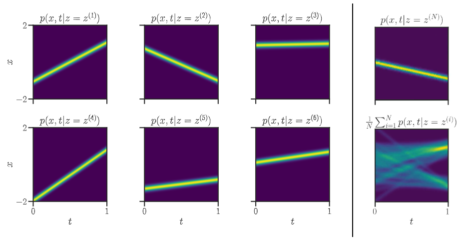
Figure 6. Visualisation of the conditional paths as linear interpolation and the convergence of empirical average towards the true marginal probabilities p_t. From [A.Gagneux et al.].
Sampling
Once the training is done, you have obtained an estimator of the velocity field \(u_t^{\theta}\), which you can use to sample data in \(p_{\textrm{data}}\) from \(p_0\). Since the relationship between the probability densities and true vector field is an ODE, data is sampled by solving the ODE, i.e. following \(u_t^{\theta}\) from \(t=0\) to \(t=1\). Any ODE solver can be used, but typically the – simplest – Euler is sufficient. Hence, the sampling procedure is the following :
- Get an initial sample \(x^{(0)}\) (a data point, see later, or sample it from the known source distribution \(p_0\))
- Define a number of steps \(T\)
- From \(x^{(0)}\), iterate \(T\) times the procedure : \(x_{t+1} = x_t + \frac{1}{T} u_t^{\theta} (x_t)\)
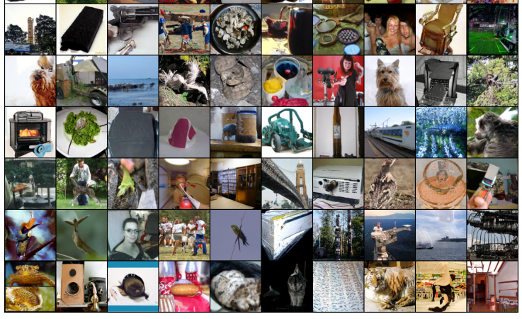
Figure 7. Examples of generated samples for a model trained on ImageNet-128. From [Y. Lipman et al.].
Summary : skeleton of code
To prove how easy and convenient (in particular compared to diffusion models) it is to train and infer a flow matching model parametrized by a neural network, we raise the challenge of coding the most condensed (and ugly) code to run training and inference of a flow matching model. It takes no more than 15 lines of code :
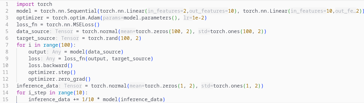
Figure 8. An implementation for the challenge of the more condensed code for a flow matching model.
A slightly longer (but way better) code to start using Flow Matching can be found here.
Few remarks and pros of Flow Matching
- Although flow matching is often presented from the perspective of data generation from Gaussian noise, one of the main advantages of flow matching, in particular in comparison with diffusion models, is that both the source and the target distributions can be sampled from real data (Figure 9). It means for instance that one can easily build a model that learns to generate CT from paired MR image.
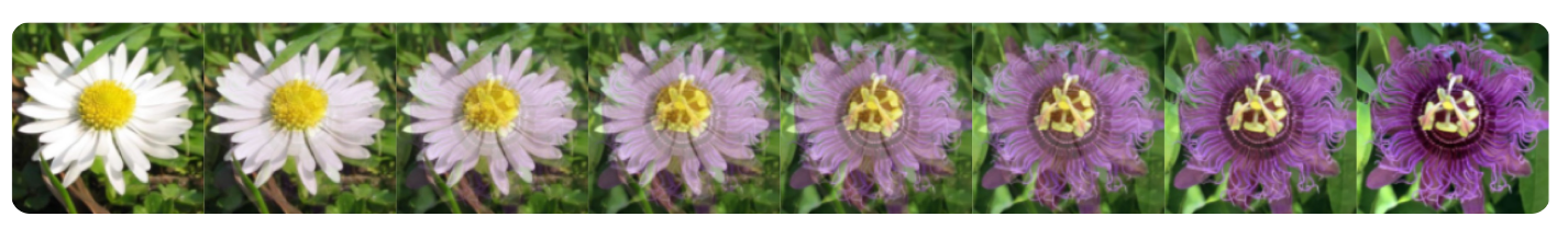
Figure 9. Example of interpolation between two distributions. From [T.Fjelde et al.].
- Another big advantage of flow matching compared to diffusion models is that the formulation of a continual problem at training allows more flexibility at inference. Indeed, in diffusion models, the number of timesteps is a fixed hyperparamters and tricks are needed to reduce the number of steps at inference. Flow matching models learn to estimate the vector field for any time \(t \in [0,1]\). At inference, one can choose to sample with any number of steps \(T\) depending desired trade-off between sampling quality and speed.
- Contrary to diffusion models, for any time \(t\), the target of parametrized estimator of the vector field \(u_t^{\theta}\) is the same (we recall that \(u_t = x_1 - x_0\)). Hence, if we want to increase the sampling speed by reducing the number of steps, the approximation we obtain should be by construction better than diffusion models.
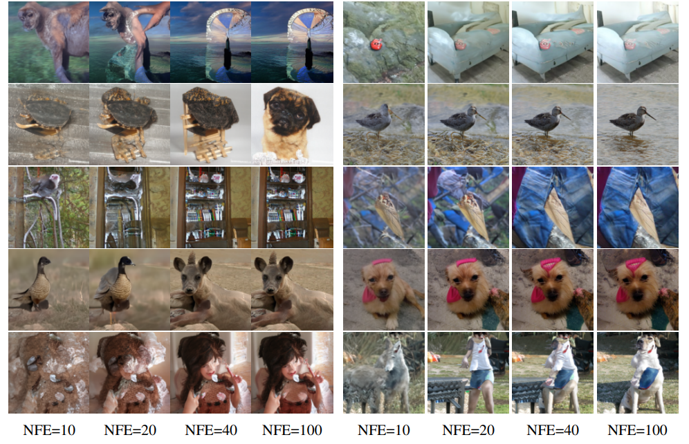
Figure 10. Generated samples from the same initial noise, but with varying number of function evaluations (NFE). From [Y. Lipman et al.].
- We did not discuss this part in this tutorial but obviously the paradigm of flow matching can be applied to conditional generation, such as image inpainting, upsampling, etc. (Figure 11).
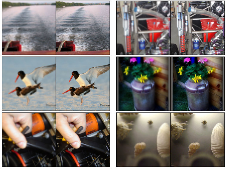
Figure 11. Examples of upsampling 64x64 -> 256x256 (conditional generation). From [Y. Lipman et al.].
Link with SDE, ODE and Diffusion Models
The link between Stochastic Differential Equation (SDE), Ordinary Differential Equation (ODE), Flow Matching and Diffusion Models would need a whole tutorial to be explained in details, but we will try to give an idea of the link between these concepts. This post have a paragraph which gives a short introduction to SDE.
To put it simply, there is a hierarchy between them : SDE is the more general concept, ODE is a particular type of SDE, Flow Matching is a sub-case of ODE and Diffusion Models is a sub-case of SDE. The forward process of a SDE is defined as follows :
\[\textrm{d}x = h(x,t)\textrm{d}t + g(t)\textrm{d}w_t\]where \(h(\cdot, t) : \mathbb{R}^D \rightarrow \mathbb{R}^D\) is the drift coefficient and \(g(\cdot) \in \mathbb{R}\). From the forward SDE process, it is possible to expressed the reversed diffusion process (solving the equation backwards in time). The functions \(h\) and \(g\) can be chosen in various ways, and their choice defines the type of model.
An ODE is a particular case of SDE where the stochasticity is removed, i.e. \(g=0\). Flow Matching is a particular case of ODE with a specific form of function \(h\), and diffusion models are a particular case of SDE. Stochasticity can be added to the original formulation of flow matching to have a non-deterministic process.
This blogpost has a nice interface to play with the many variants of Flow Matching (see their interactive Figure 16).
To go further : advanced concepts
This last part of the tutorial aims to give a broad view of the range of open research topics on flow matching, and some of the variants of the initial formulation that have been introduced since 2022.
Improve probability paths with data pairing
The training of a model of flow matching relies on an empiric (average on a batch of training data) approximation of the expectation between the true velocity fields and the estimated one. As presented in the training algorithm, at each step of the stochastic gradient descent, we randomly sample a batch of paired data from the source and target distributions. This results in crossing paths and suboptimal learnt probability paths, as shown in the Figure below (left). One way to solve this problem is to use optimal transport to create the pairs of data when a batch of samples from the source and target distributions at training (right parts of the Figures below).
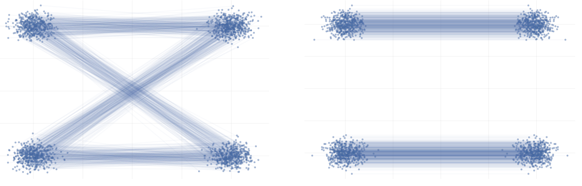
Figure 12. Learnt probability paths between two mixtures of gaussians with normal sampling (left) and with OT sampling (right). From [T.Fjelde et al.].
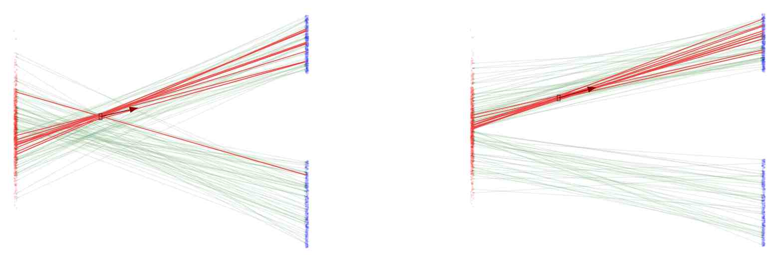
Figure 13. Another example of difference between normal sampling (left) and with OT sampling (right). From [A.Gagneux et al.].
Non-Euclidean Flow Matching
There are many attempts to extend Flow Matching from \(\mathbb{R}^D\) to general Riemannian manifolds (Figure 14). An example of work has been presented in this post.
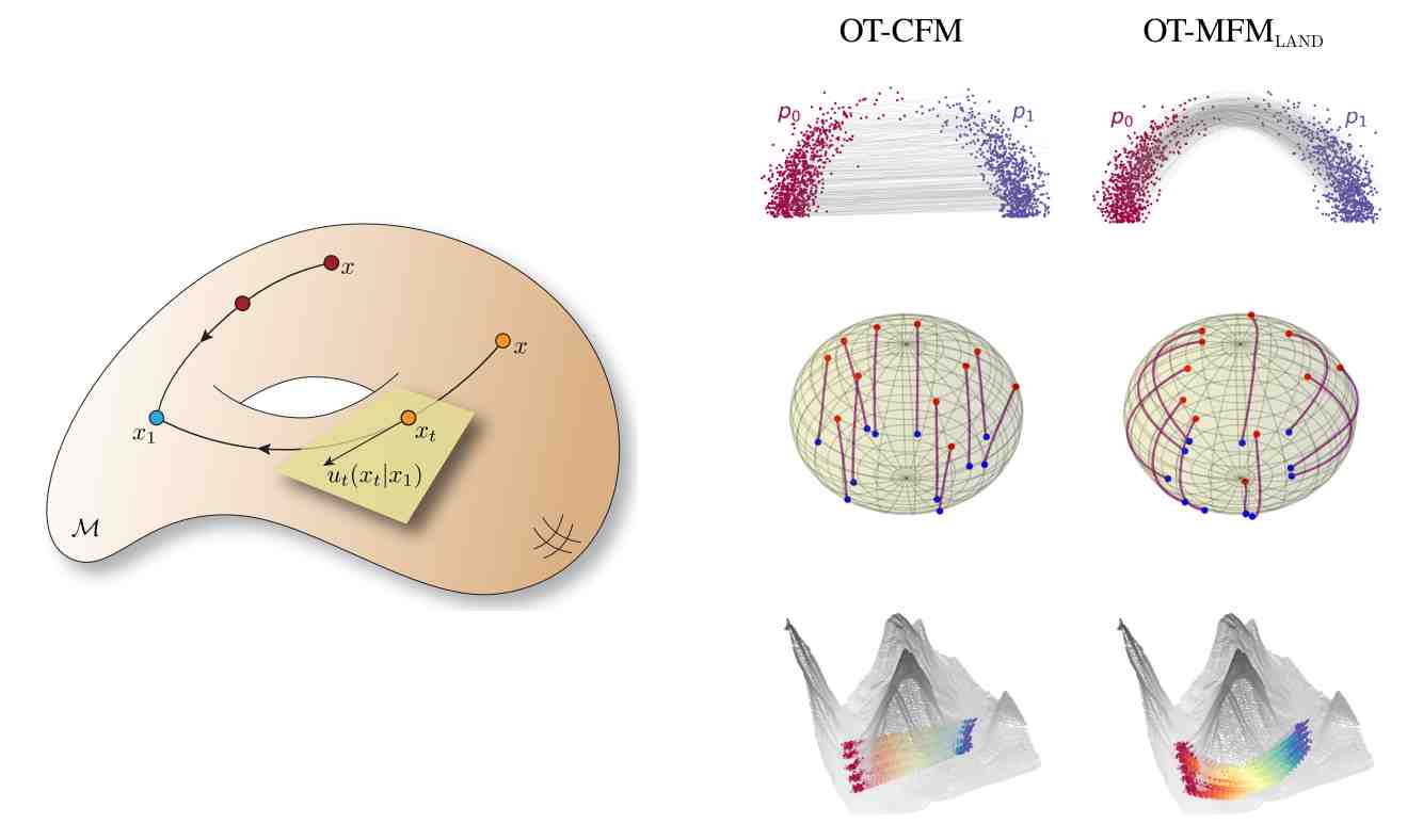
Figure 14. Illustrative examples of Riemannian Flow Matching.
Flow Matching on Discrete Sets
Another field of investigation on Flow Matching is the extension of its formulation to discrete sets (Figure 15). It is of great interest for text generation and could be the next state-of-the-art paradigm for Large Language Models.
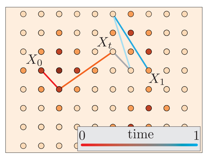
Figure 15. Illustrative examples of Flow Matching on a discrete set.
Conclusion
Flow Matching is the new state-of-the-art paradigm for image generation and data distribution estimation. It relies on the learning of vector fields and conditional probability paths to transform the source distribution into the target distribution. It allows to solve the constraints of continuous normalizing flows, which were limitating to scale them to high dimension problems. Compared to diffusion models, Flow Matching is simpler and has several advantages, in particular the flexibility of time steps at inference and the possibility to build paths between two arbitrary distributions.
References
-
Y. Lipman et al., Flow Matching for Generative Modeling, NeurIPS 2024. ↩